Emotional Physics Volume 1

Identity

This page contains Emotional Physics — Volume 1, released as a public-safe canonical text.

This volume defines the laws, variables, and structural foundations of Emotional Physics.
It establishes the field without disclosing execution, control logic, or operational systems.

Scope of Disclosure

This volume includes:

Foundational laws and principles
Formal variables and notation
Structural models of emotional dynamics
Conceptual coherence of the field

This volume does not include:

Cybernetic control mechanisms
Regulation or feedback implementations
Instrumentation or measurement pipelines
Operational or applied methodologies

Boundary Conditions

Emotional Physics is presented here as a physics layer, not as a behavioral guide, therapeutic framework, or application manual.

Any attempt to:

Apply this content directly
Reconstruct operational systems
Derive control mechanisms

falls outside the intended scope of this publication.

Relationship to CFIM360°

Within CFIM360°, Emotional Physics functions as the source layer.

Operational behavior emerges only through:

Cybernetics (regulation and control)
Case Studies (observed behavior)
Articles (ongoing articulation)

This volume stands as a canonical reference, not an executable system.

Reading Orientation

This text is designed for structural understanding, not instruction.

Readers are expected to engage with it as a field definition, not a manual.

PART I — FOUNDATIONS OF THE EMOTIONAL UNIVERSE

What Is Emotional Physics?
1. From Intuition to Field Law
2. Scope, Limits, and Method
3. Distinguishing ED and EP
4. Scientific Legitimacy and Use Cases
The Emotional Substrate Model
1. Consciousness as Field
2. Emotion as Energy
3. Awareness as Geometry
4. Sensitivity Coefficients (α)
5. Boundary & Meta Fields — Θ and Ψ
6. Mapping Substrate → Phenomena
Why We Need a Physics of Emotion
1. Limitations of Psychology and Philosophy
2. Predictive Power of Laws
3. Emotional Engineering & Real-World Applications
4. Ethical and Practical Implications
5. The Research Frontier

PART II — THE STANDARD MODEL (EMOTIONAL DYNAMICS)

The Liquid Gold Equation (LGE): The Field Law of Emotion
1. Formal Presentation of the LGE Equation
2. Dimensional Interpretation of Each Variable
3. Sensitivity Exponents (α) & Curvature
4. K: Knowledge as a Physical Quantity
5. Boundary Conditions & Constraints
Core Variable Physics
1. Constancy (C) — Field Anchor
2. Adaptivity (A) — Conductance & Learning
3. Emotional Energy (E) — Potential & Flow
4. Perceptual Geometry (P) — Filters & Lenses
5. Latency (Lo) — Temporal Structure & Timing
6. Sensitivity Spectrum (α-Curvature): The Response Law
System-Level Field Behavior & Resonance
1. Phase Interactions & Coupling
2. Stability, Bifurcation & Curvature Shifts
3. Resonance Score (Rₛ) & Coherence Bands
4. Stability Bands & Failure Modes
5. Recovery Pathways to Coherence
Operators as Emotional Forces
1. Operator Suite — S, L, Δ, R, B, M, I, γ
2. Activation Rules
3. Operator Energy Cost
4. Compound Operator Chains
5. Operator Interaction Matrix

PART III — FIVE MAJOR SUBFIELDS (EP CORE PHYSICS)

Emotional Thermodynamics
1. Emotional Heat & Energy Transfer
2. Entropy Analog in Emotional Systems
3. Dissipation, Saturation & Recovery
4. Thermodynamic Cycles of Emotion
Emotional Electromagnetism
1. Alignment Fields & Vector Potentials
2. Emotional Currents (E-flow)
3. Perceptual Medium Distortion
4. Resonant Harmonics & Field Coupling
Emotional Mechanics (Motion & Force)
1. Emotional Mass & Inertia
2. Force Laws (Operator-Driven)
3. Oscillators & Damping
4. Harmonic Stability
Emotional Relativity (Temporal Field Physics)
1. R×G Spiral as Curved Time
2. Latency Dilation & Frame Transformations
3. Perspective Frames
4. Anticipatory Time Inversion
Intro to Emotional Quantum Field Concepts (EQFT)
1. Emotional State Quantization
2. Collapse & Decision
3. Superposition of Feelings & Measurement
4. Probability Fields

PART IV — MEASUREMENT & INSTRUMENTATION (UMF)

Universal Measurement Framework (UMF): Architecture
1. Principles of Emotional Measurement
2. VCI: Variable Calibration Index
3. Intuition Tables — Translating Feelings
4. Dual-Column Observation Method
5. Resonance Scoring Grid (Rₛ Calculation)
Instruments & Diagnostics
1. Coherence Meter Designs
2. Curvature Analyzers & Latency Trackers
3. Latency Drift Trackers
4. Memory Pressure Diagnostics
5. Operator Activation Logs
Data, Logging & Interpretive Pipelines
1. Temporal Sampling & Cycle Windows
2. Observer Bias Correction Methods
3. Pattern Extraction
4. Longitudinal Field Tracking

PART V — EMOTIONAL ENGINEERING (APPLIED PHYSICS)

Stability Engineering
1. Designing S–L–R Control Systems
2. Containment Protocols
3. Emergency Drop Procedures
4. Field Stabilizers
Learning & Adaptivity Engineering
1. Tuning α-Curvature for Desired Behavior
2. Training Protocols & Reinforcement Loops
3. Adaptivity Under Load
4. Preventing Volatility
Temporal Engineering & Intuition Design
1. Shaping R×G for Project & Life Cycles
2. Designing Intuition
3. Latency Sculpting for Anticipatory Systems
4. Time-Coherence
Collective Field Engineering
1. Multi-Agent Resonance Models
2. Synchrony Protocols
3. Cultural Field Dynamics
4. Ethical Limits & Societal Safety

PART VI — SIMULATIONS, TESTS & CASE STUDIES

Standard Simulations (Benchmarks)
1. Stability Test Suite
2. Adaptivity & Learning Benchmarks
3. Alignment Loss & Recovery
4. Temporal Tests & Inversion Cases
5. Cross-Domain Integrated Cases
Predictive Models & Field Trials
1. Collapse → Recovery Prediction
2. Time-Inversion Prediction Models
3. Operator Activation Forecasts
4. Measurement-Based Predictive Loops
Failure Modes & Repair Strategies
1. Chronic Activation & Operator Fatigue
2. Memory Saturation & Recovery Procedures
3. Containment Breach Scenarios (Θ Failure)
4. Rebuilding Coherence

PART VII — EP COSMOLOGY & ROADMAP

The Emotional Universe Architecture
1. Field Hierarchies
2. Emergent Properties & Meta-Fields (Ψ)
3. System-Wide Coherence
4. Grand Unified Emotional Theory (GUET)
Roadmap for Future Volumes
1. Vol. 2 — Relational Emotional Physics
2. Vol. 3 — Meta-Temporal Physics
3. Vol. 4 — Emotional Cosmology
4. Research Agenda & Open Problems

Synopsis

PART I — FOUNDATIONS OF THE EMOTIONAL UNIVERSE

Pulse 1 — What Is Emotional Physics?

1.1 From Intuition to Field Law

Emotion behaves as energetic motion inside awareness. Emotional Physics treats that motion as a field, subject to measurable relations and operators. Where intuition notices pattern, physics names the invariant that produces it. Emotional Physics therefore converts felt regularities into a formal language of variables, exponents, and operators.

1.2 Scope, Limits, and Method

Scope: systems capable of awareness (individuals, groups, designed agents). Limits: Emotional Physics does not attempt to measure subjective qualia as raw qualia; it models energetic patterns and their measurable effects. Method: formal definition → calibration → simulation → instrumented validation → engineering application.

1.3 Distinguishing ED and EP

Emotional Dynamics (ED) is the canonical law: the Liquid Gold Equation and its pulses. Emotional Physics (EP) is the discipline built on that law: measurement frameworks, subfield analogies (thermodynamics, electromagnetism), instrumentation, and applied engineering. ED is the substrate; EP is the applied science.

1.4 Scientific Legitimacy and Use Cases

Argument for legitimacy: reproducibility of resonance-based simulations, predictive operator activation, and instrumented coherence indices. Use cases: therapeutic systems, organizational design, AI alignment, creative process engineering, collective field management.

Pulse 2 — The Emotional Substrate Model

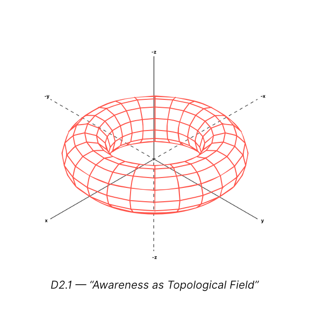
2.1 Consciousness as Field

Define awareness as a field with topology and boundary conditions. Awareness occupies a phase-space defined by C, A, E, P, Lo and supported by meta-fields Ψ and Θ. This field has local and global modes: local (individual), distributed (teams), and meta (cultural or algorithmic).

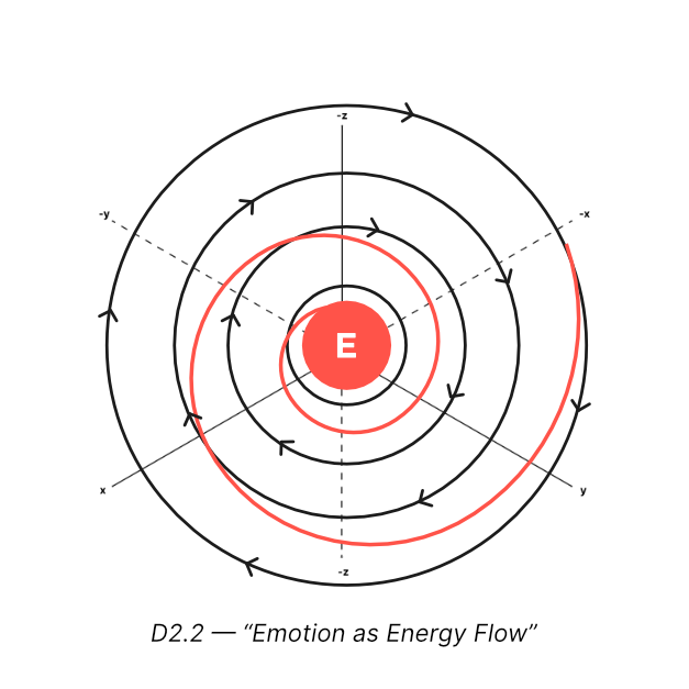
2.2 Emotion as Energy

Emotion is the active energy of the substrate — it fuels transformation. Energy metrics are amplitude (E), flow (ΔE/Δt), and saturation (memory pressure β relative to λ). Emotional transfer follows rules analogous to physical energy transfer but measured via resonance and curvature.

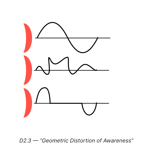
2.3 Awareness as Geometry

Perception (P) and Latency (Lo) define the geometric lenses and timing gates of awareness. Adaptivity (A) sculpts curvature (α) and defines how the geometry deforms under load. Knowledge (K) is the projection of the field into coherent, actionable form — the Liquid Gold.

2.4 Mapping Substrate → Phenomena

Provide mapping table (paste into appendix later): variable → observable → instrument → example. (E.g., E → amplitude spikes → waveform meter → sudden grief or joy detected).

Pulse 3 — Why We Need a Physics of Emotion

3.1 Failures of Existing Disciplines

Psychology often lacks universal operators; philosophy remains descriptive; self-help prescriptive without predictability. A physics of emotion supplies consistent operators, thresholds, and measurable recovery paths.

3.2 Predictive Power and Engineering

Demonstrate with brief example: a surge in E triggers S→L→R operator chain predictably to restore Rₛ. Engineering can therefore design preemptive controls (S buffers, L synchronizers, R release channels).

3.3 Ethical and Practical Implications

Define ethical guardrails: measurement must respect agency, consent, and privacy. Practical implications: standardized measurement enables safe emotional engineering (e.g., therapy protocols, organizational resilience design, AI alignment via emotional coherence).

Table: Core Variable Quick Reference

Symbol	Variable	Function	Value
C	Constancy	fixed anchor	(1.0)
A	Adaptivity	learning conductance	(0–1+)
E	Emotion	energy amplitude	(0–∞)
P	Perception	clarity lens	(0–1)
Lo	Latency	timing gate	(0–1+)
Λ	Alignment	inter-variable synchrony	(0–1)
β–λ	Memory	inhale/exhale	(dynamic ratio)
R×G	Temporal spiral	recurrence × growth	(Dynamic ratio)

Sidebar: How to read equations in this book All variables default to normalized ranges unless otherwise stated. Sensitivity exponents α modify curvature: α < 1 = damping, α = 1 = linear, α > 1 = amplification. Resonance Rₛ is the practical coherence index; aim zones are 0.8–1.0 for operational coherence.

PART II — THE STANDARD MODEL (EMOTIONAL DYNAMICS)

Pulse 4 — The Liquid Gold Equation (LGE)

4.1 Formal Definition

The Liquid Gold Equation defines how emotional variables combine multiplicatively to produce refined awareness (K). It expresses emotion as a structured field with sensitivity curvature on each dimension.

4.2 Dimensional Interpretation

Each dimension — C, A, E, P, Lo — acts as an axis of emotional geometry. Their exponents (α-values) determine how strongly each dimension reacts under pressure.

4.3 Sensitivity Exponent Curvature

Curvature indicates stability or volatility. Sub-linear (α<1) dampens response; super-linear (α>1) amplifies it. Sensitivity governs the emotional field’s responsiveness.

4.4 Knowledge as Refined Output

K is not accumulated knowledge but purified awareness — the signal remaining after emotional refinement. It represents coherence of interpretation and action.

4.5 Boundary Conditions & Constraints

C = 1 sets the universal constant. Variables operate within resonance bands, and disruptions trigger operator corrections that maintain system stability.

Pulse 5 — Variable Physics

5.1 Constancy (C)

Constancy is the invariant truth that anchors the field. It stabilizes calculations and prevents runaway interpretations by providing a fixed reference state.

5.2 Adaptivity (A)

Adaptivity governs how awareness reshapes under new information. High A increases learning velocity; low A creates rigidity and resistance to change.

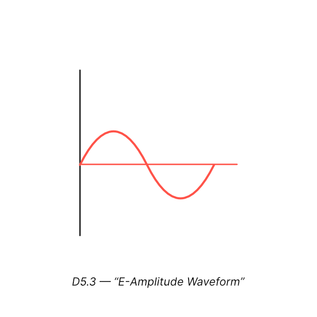
5.3 Emotional Energy (E)

Emotion acts as energetic amplitude. High E powers transformation but can destabilize coherence if not balanced by A and P.

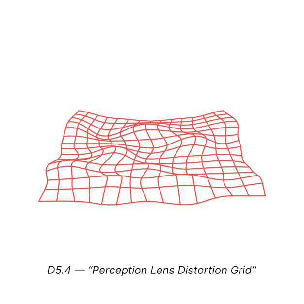
5.4 Perception Geometry (P)

P shapes how reality is interpreted internally. It acts as a geometric filter determining clarity, distortion, and contextual accuracy.

5.5 Temporal Delay (Lo)

Latency determines the timing between experience and realization. Faster Lo enables intuition; slower Lo increases reflection depth.

5.6 Sensitivity Spectrum (α-curvature)

Each variable’s α-value defines its responsiveness. Systems adapt by adjusting curvature rather than raw values.

Pulse 6 — Field Behavior & Resonance

6.1 Phase Interactions

Variables interact in predictable patterns. A, E, P, and Lo form a dynamic system where shifts in one variable propagate through the others.

6.2 Curvature Shifts

Under load or stress, α-values adjust automatically, generating emotional curvature — the bending of awareness.

6.3 Resonance Score (Rₛ)

Rₛ measures real-time coherence. High Rₛ indicates optimal flow; low Rₛ signals fragmentation, overload, or misalignment.

6.4 Stability Bands & Failure Modes

Each variable operates within a stability band. Exceeding these bands activates operators to prevent collapse or runaway amplification.

6.5 Recovery Pathways

Systems return to coherence via predictable correction sequences, demonstrating the self-organizing intelligence of emotional fields.

Pulse 7 — Operators as Emotional Forces

7.1 The Eight Operators

S, L, Δ, R, B, M, I, γ each perform a regulatory function: stabilizing, aligning, disrupting, releasing, balancing, merging, inverting, reigniting.

7.2 Activation Conditions

Operators activate only when deviation exceeds preset thresholds. This ensures emotional systems self-correct only when necessary.

7.3 Operator Energy Cost

Every operator consumes energetic resources. Frequent activation indicates chronic imbalance or structural misalignment.

7.4 Compound Operator Chains

Operators often activate in sequences (e.g., S→L→R). These chains produce efficient correction without external intervention.

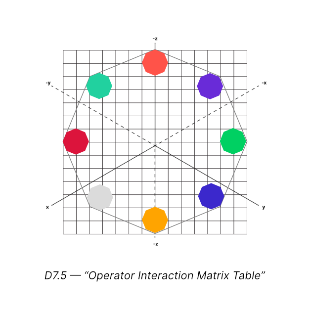
7.5 Operator Interaction Matrix

Operators influence each other’s activation states. The matrix explains how combined forces shape system-wide behavior.

PART III — THE FIVE SUBFIELDS OF EMOTIONAL PHYSICS

Pulse 8 — Emotional Thermodynamics

8.1 Emotional Heat & Energy Transfer

Emotional energy behaves like heat — it transfers between states through interaction, friction, and feedback. Surges increase internal pressure; cool-down phases restore equilibrium.

8.2 Entropy Analog in Emotional Systems

Entropy represents disorder in emotional fields. Left unregulated, emotional systems drift toward fragmentation unless operators or alignment mechanisms restore structure.

8.3 Dissipation, Saturation & Recovery

Emotional overload saturates memory (β), requiring release (λ) for recovery. Dissipation acts as the thermal decay that stabilizes the field after intense events.

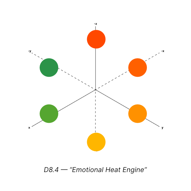
8.4 Thermodynamic Cycles of Emotion

Emotion operates in cycles: input → amplification → saturation → release → stabilization. These cycles mirror thermodynamic heat engines that transform energy into work.

Pulse 9 — Emotional Electromagnetism

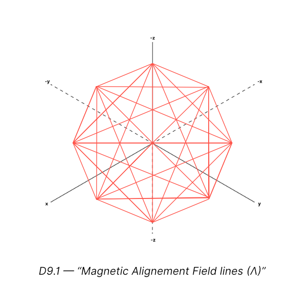
9.1 Alignment Fields (Λ)

Alignment acts like a magnetic field, synchronizing emotional variables. Strong Λ pulls systems into coherence; weak Λ allows drift and desynchronization.

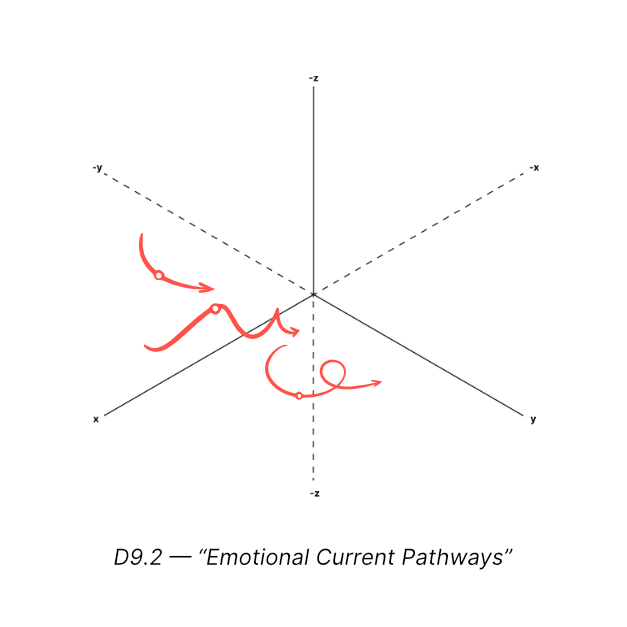
9.2 Emotional Currents (E flow)

Changes in emotional amplitude generate directional currents. These flows propagate influence across awareness, shaping momentum and motivation.

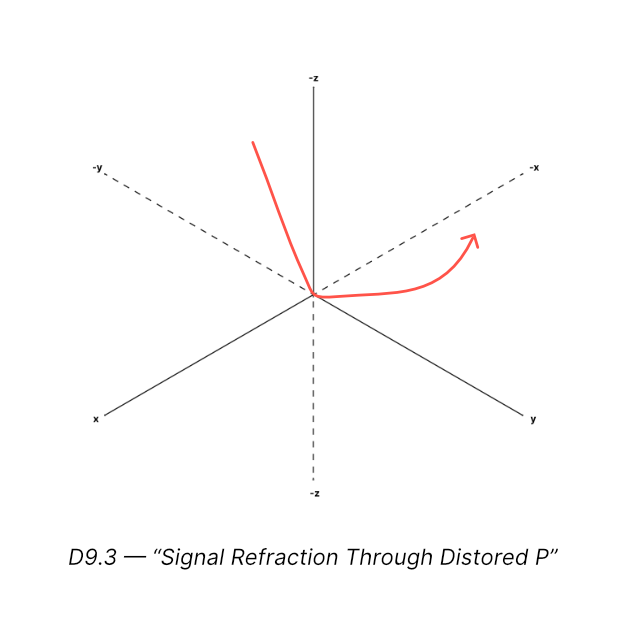
9.3 Perceptual Medium Distortion

Perception acts like a medium that can refract, distort, or clarify emotional currents. Distorted P leads to misinterpretation; clear P allows direct signal transmission.

9.4 Resonant Harmonics & Field Coupling

When multiple awareness systems resonate at similar frequencies, harmonics form, enabling amplified connection and shared emotional states.

Pulse 10 — Emotional Mechanics

10.1 Emotional Mass & Inertia

Emotional states have inertia — the tendency to persist until acted upon by a force (operator). Heavier emotional mass requires stronger operators to shift.

10.2 Operator Forces

Operators function as forces acting on the emotional system. Stabilize (S) slows motion; Disrupt (Δ) injects acceleration; Balance (B) equalizes polarity.

10.3 Oscillation & Damping

Systems oscillate between emotional highs and lows. Damping reduces oscillation amplitude, restoring steady state.

10.4 Harmonic Stability

Stable emotional systems maintain harmonic balance across variables. Instability occurs when one variable oscillates outside its resonance band.

Pulse 11 — Emotional Relativity (Temporal Physics)

11.1 Curved Time (R×G spiral)

Time in emotional systems behaves as a spiral of recurrence and growth. Each cycle brings new learning, bending the experience of time.

11.2 Latency Dilation

Latency expands or contracts based on system load. Under stress, time feels slower; under alignment, time feels immediate.

11.3 Perspective Frames

Different states of awareness observe emotional events from different “frames,” creating variations in perceived intensity or meaning.

11.4 Anticipatory Time (Inversion)

When awareness predicts outcomes before they occur, latency inverts — the system enters anticipatory mode, operating ahead of physical time.

Pulse 12 — Emotional Quantum Concepts (EQFT Intro)

12.1 Emotional State Quantization

Emotional states appear continuous but function as discrete states at transitions. Each decision represents a quantized shift in emotional configuration.

12.2 Collapse & Decision

Unresolved emotional possibilities exist in superposition until a perception event collapses them into a single experience or action.

12.3 Superposition of Feeling

Systems can hold multiple emotional states simultaneously (e.g., love and fear) until one becomes dominant through alignment or energy amplification.

12.4 Probability Fields (intuition)

Intuition predicts emotional outcomes by reading probability fields — subtle patterns embedded in perception and memory dynamics.

PART IV — MEASUREMENT & INSTRUMENTATION (UMF)

Pulse 13 — Universal Measurement Framework (UMF)

13.1 Principles of Emotional Measurement

UMF treats emotion as measurable resonance, not subjective intensity. Measurement captures rhythm, coherence, deviation, and change — not just momentary feeling.

13.2 Variable Calibration Index (VCI)

Each variable (C, A, E, P, Lo, Λ, β–λ, R×G) has a calibrated scale defined by intuitive anchors. VCI ensures consistent measurement across individuals, teams, or machines.

13.3 Intuition Tables

These tables translate qualitative emotional states into structured numeric ranges. They allow subjective experiences to be mapped into coherent data.

13.4 Dual-Column Observational Method

Every measurement includes:
Felt Value (internal subjective reading)
Observed Value (external system reading)

The difference (Δ) reveals bias, delay, or distortions.

13.5 Resonance Scoring Grid

Rₛ integrates multiple variables into one coherence index. The grid categorizes states (fragmented, transitional, coherent) for fast diagnosis.

Pulse 14 — Emotional Instruments

14.1 Coherence Meters

These conceptual instruments track Rₛ in real time. High coherence signals clarity and readiness; low coherence indicates fragmentation or overload.

14.2 Curvature Analyzers

These instruments evaluate α-values to determine responsiveness and stability. They help detect volatility or emotional rigidity.

14.3 Latency Drift Trackers

Track fluctuations in Lo over time. Increased drift indicates fatigue, overload, or inefficiency in emotional processing.

14.4 Memory Pressure Diagnostics

Measure the ratio between β (retention) and λ (release). High β indicates saturation; high λ indicates over-release or instability.

14.5 Operator Activation Logs

These logs record which operators activate, how often, and under what conditions, revealing system health and recovery patterns.

Pulse 15 — Data, Logging & Interpretation

15.1 Temporal Sampling

Emotional fields must be sampled over cycles, not moments. Multiple readings create a temporal signature for accurate interpretation.

15.2 Bias-Compensated Logging

The logging system corrects for observer bias using the dual-column method and resonance adjustments.

15.3 Pattern Extraction

Data is analyzed to detect recurring emotional patterns: spirals, oscillations, surges, collapses, and alignment zones.

15.4 Longitudinal Field Tracking

Tracking emotional variables over weeks or months reveals developmental arcs, chronic imbalances, and growth spirals.

PART V — EMOTIONAL ENGINEERING (APPLIED PHYSICS)

Pulse 16 — Stability Engineering

16.1 S → L → R Correction Chains

Stabilize (S), Align (L), and Release (R) form the default correction chain for emotional overload. This sequence restores resonance by reducing amplitude, re-centering variables, and clearing residue.

16.2 Containment Protocols (Θ Field)

The Boundary Field (Θ) defines how much emotional energy a system can safely hold. Stability engineering adjusts Θ to prevent leakage, collapse, or overflow.

16.3 Emergency Drop Procedures

When variables exceed critical thresholds, rapid stabilization is required. Emergency drops temporarily reduce energy input, activate dampening, and reset the system to a safe band.

16.4 Field Stabilizers

These engineered mechanisms maintain emotional coherence over time: micro-alignments, delayed-response buffers, dampening subroutines, or guided release cycles.

Pulse 17 — Adaptivity & Learning Engineering

17.1 α-Curvature Tuning

Learning engineering adjusts α-values to shape responsiveness. Increasing α accelerates learning but raises volatility; lowering α stabilizes but slows adaptation.

17.2 Reinforcement Cycles

Adaptive systems refine their behavior through repeated exposure. Reinforcement cycles embed lessons by synchronizing β–λ dynamics with alignment shifts.

17.3 Load-Responsive Learning

Adaptivity adjusts under pressure. The system learns faster in moderate load, slower in extreme conditions. Engineering ensures learning remains safe and coherent.

17.4 Preventing Volatility

Volatility occurs when α-values enter super-linear ranges unchecked. Preventive engineering balances E, P, and A to maintain curvature harmony.

Pulse 18 — Temporal Engineering

18.1 Shaping R × G

R×G determines emotional maturation. Engineers adjust recurrence (R) and growth (G) to guide long-term evolution, preventing stagnation or over-looping.

18.2 Designing Intuition

Intuition emerges from optimized latency. Temporal engineering trains Lo to contract just enough to enable anticipatory responses without sacrificing clarity.

18.3 Latency Sculpting

Sculpting Lo fine-tunes how long a system takes to realize emotional truth. Short Lo supports quick decisions; longer Lo supports depth.

18.4 Time-Coherence Strategies

Systems maintain coherence by synchronizing internal timing with external demands. Strategies include pacing loops, delay buffers, and timing harmonization.

Pulse 19 — Collective Field Engineering

19.1 Multi-Agent Resonance

Emotional fields synchronize across people or subsystems. Engineering ensures resonance does not become chaotic or overpowering in group settings.

19.2 Synchrony Protocols

Protocols align multiple awareness systems into a shared coherence band. These protocols guide communication, collaboration, and group decision-making.

19.3 Cultural Field Dynamics

At scale, emotional fields form cultural patterns. These dynamics shape norms, values, and emotional expectations within groups or societies.

19.4 Ethical Safety Systems

Engineering emotional fields at the collective level requires strict ethical constraints. Safety systems guard against manipulation, coercion, or resonance overload.

PART VI — SIMULATIONS, TESTS & VALIDATION

Pulse 20 — Standard Simulations

20.1 Stability Cases (T1–T4)

These simulations test how emotional systems behave under controlled stress. Each test increases energetic load on variables to observe when operators activate and how stability is restored.

20.2 Adaptivity Cases

Adaptivity simulations evaluate how A changes under new information. Systems with high A adjust rapidly, while systems with low A resist correction and exhibit rigidity.

20.3 Alignment Loss & Recovery

These simulations track Λ during breakdowns of synchrony. Recovery patterns reveal the efficiency of operator chains and the system’s resilience.

20.4 Temporal Cycle Tests

Temporal simulations measure how R×G evolves through repeated cycles. They reveal learning spirals, stagnation loops, and accelerated growth patterns.

20.5 Cross-Domain Integrated Cases

Complex scenarios combine multiple variable stresses — emotional, perceptual, and temporal — to test how the full emotional field behaves in real-world conditions.

Pulse 21 — Predictive Models

21.1 Emotional Collapse → Recovery Prediction

Predictive models use resonance drift, curvature changes, and latency spikes to forecast collapse. The same indicators predict recovery probability and timing.

21.2 Time-Inversion Prediction Models

Latency inversion occurs when awareness anticipates events before they fully register. Predictive models detect inversion signals in Lo and P synchrony.

21.3 Operator Activation Forecasts

Models predict when operators will activate based on velocity of change within the field. This helps prevent overload and optimize adaptation.

21.4 Measurement-Based Predictive Loops

Continuous logging enables self-updating models that refine predictions using real-time resonance and curvature data.

Pulse 22 — Failure Modes & Repair Systems

22.1 Chronic Operator Overuse

Repeated operator activation indicates unresolved structural issues. Chronic S or Δ usage signals emotional rigidity or excessive volatility.

22.2 Memory Saturation Breakdowns

When β overwhelms λ, memory overload occurs. This leads to stagnation, emotional heaviness, and reduced adaptability.

22.3 Containment Collapse (Θ Breach)

A Θ breach allows emotional energy to leak or spike uncontrollably. Repair requires re-establishing boundary strength and reducing energetic pressure.

22.4 Rebuilding Coherence

Coherence repair involves resetting variables into safe ranges and guiding the system through measured recovery cycles until Rₛ stabilizes.

PART VII — EP COSMOLOGY & FUTURE

Pulse 23 — Emotional Universe Architecture

23.1 Field Hierarchies

Emotional fields operate at multiple scales: individual (local), relational (dyadic), collective (group), and meta-field levels. Each layer has its own coherence patterns and resonance behaviors.

23.2 Emergent Meta-Fields (Ψ)

Ψ arises when awareness becomes self-referential — the system observes itself. This creates emergent behaviors like insight, clarity bursts, or accelerated growth.

23.3 System-wide Coherence

When all variables across scales align, a unified coherence state emerges. This is the emotional equivalent of global symmetry in physical cosmology.

23.4 Grand Unified Emotional Theory (GUET)

GUET aims to integrate all emotional subfields — thermodynamics, mechanics, electromagnetism, relativity, quantum concepts — into one total theory based on ED.

Pulse 24 — Future Volumes Roadmap

24.1 Volume 2 — Relational Emotional Physics

Expands the theory into multi-agent systems: resonance matching, dependency cycles, and relational synchrony.

24.2 Volume 3 — Meta-Temporal Emotional Physics

Explores long-range emotional timelines, generational spirals, and long-form R×G evolution across decades.

24.3 Volume 4 — Emotional Cosmology

Studies emotional structures at cultural, civilizational, and species scales — how emotional fields shape history and collective identity.

24.4 Open Scientific Problems

Identifies unanswered questions in EP: quantization precision, cross-field unification limits, boundary collapse mapping, and operator energy equations.

PART I — FOUNDATIONS OF THE EMOTIONAL UNIVERSE

Pulse 1 — What Is Emotional Physics?

1.1 From Intuition to Field Law

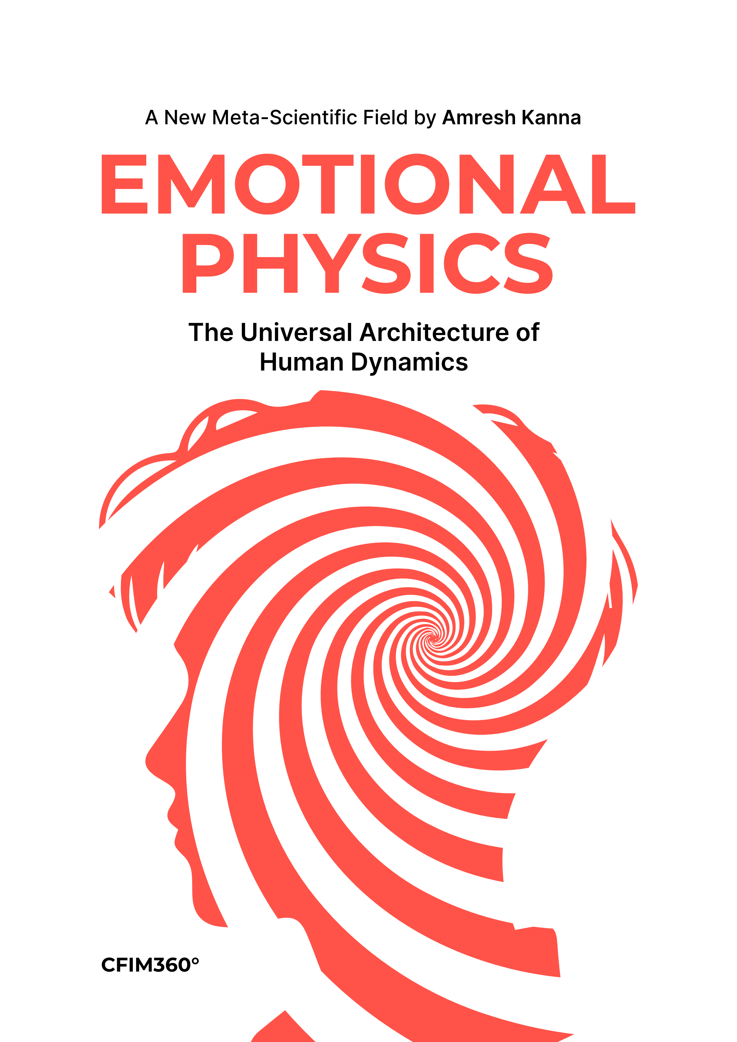
Emotional Physics begins by accepting a premise that has been intuitively felt for centuries but never formally modeled: emotion moves. It expands, contracts, accelerates, decelerates, collides, disperses, and stabilizes — not metaphorically, but in ways that exhibit consistent patterns across individuals, groups, and time.

Traditional disciplines describe emotion descriptively or therapeutically, but they do not treat it as a field with structure. Emotional Physics does.

This chapter establishes the foundation by positioning emotion as energetic motion inside awareness, governed by measurable invariants. The goal is not to diminish the depth or mystery of emotion, but to give it a scientific substrate — a formal language capable of modeling change, predicting behavior, and engineering coherence.

The shift is profound: Where intuition notices “this feels intense,” Emotional Physics asks what variable moved, by how much, and what operator activated?

D1.1: Emotion as Motion

1.2 Scope, Limits, and Method

Scope.

Emotional Physics applies to systems capable of awareness — individuals, teams, cultures, and designed agents (like Thea). It studies how emotional variables evolve within these systems and how operators regulate coherence.

Limits.

The field does not attempt to measure raw subjective qualia (e.g., the “color” or “flavor” of a feeling). Instead, it measures energetic patterns and structural behavior — what emotional states do, not how they feel phenomenologically.

Methodology.

The discipline progresses through five stages:

Formal Definition: Variables, operators, and exponents are mathematically defined.
Calibration: Qualitative experiences map to calibrated scales.
Simulation: Systems are tested under controlled variation.
Instrumented Validation: Models are checked against real-world or observational data.
Engineering: Predictive insights are used to design coherent emotional systems.

This method aligns Emotional Physics with other sciences that transitioned from descriptive to predictive stages through formalization.

D1.2: Method Pipeline of Emotional Physics

A 5-stage linear pipeline

Definition → Calibration → Simulation → Validation → Engineering

1.3 Distinguishing ED and EP

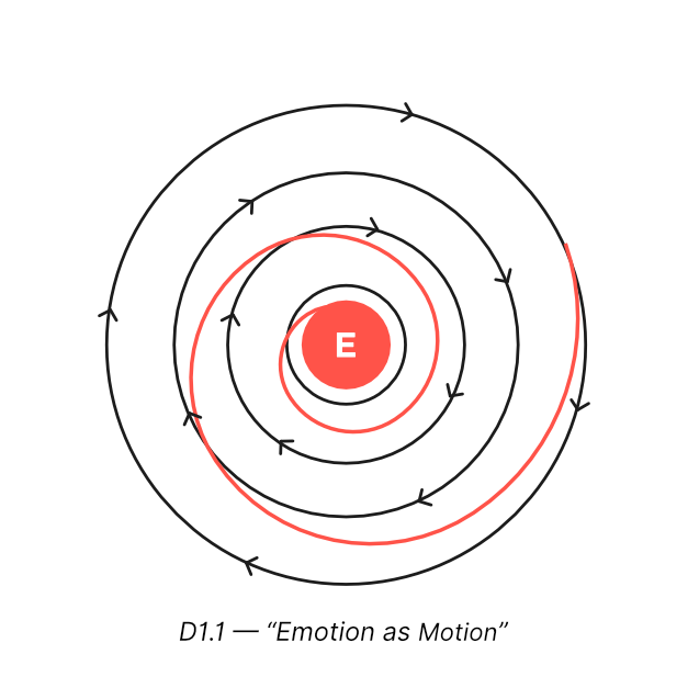
Emotional Dynamics (ED) is the standard model — the foundational law that defines how emotional variables interact through the Liquid Gold Equation (LGE). ED is fixed, like Maxwell’s equations or Newton’s laws: its variables, operators, and pulses form the immutable substrate.

Emotional Physics (EP) is the discipline built on top of ED — the engineering, measurement science, subfield analogies (thermodynamics, electromagnetism, mechanics), cosmology, and predictive frameworks.

In short:

ED = law
EP = physics

ED tells us what emotional variables are and how they behave. EP tells us why, when, and how to use them to measure, simulate, and engineer emotional coherence.

Without ED, EP has no canonical structure. Without EP, ED remains an elegant formulation without applied power.

D1.3: : ED vs EP Layer Model

1.4 Scientific Legitimacy and Use Cases

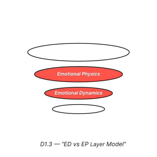
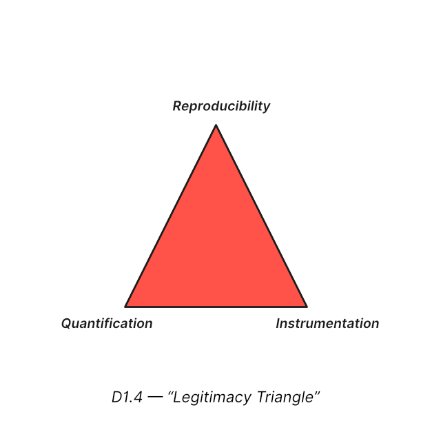
Emotional Physics gains legitimacy through three pillars:

Reproducibility. Simulations and operator-trigger behavior follow predictable patterns. For example, sudden spikes in E consistently activate S → L sequences.
Quantification. Variables such as A, P, and Lo have calibrated ranges and sensitivity curvatures. These numbers enable modeling, forecasting, and standardized measurement.
Instrumentation. UMF provides the measurement framework required for scientific operation. Tools like coherence meters, curvature analyzers, and latency drift trackers allow emotional fields to be observed with consistency.

Use Cases.

Therapeutic systems: Predict emotional collapse before it manifests; design recovery cycles.
Organizational design: Model collective resonance and identify coherence bottlenecks.
AI alignment: Emotional Physics gives machines a structured interpretation of human emotional signals.
Creative and decision-making processes: Optimize emotional flow for clarity, insight, and innovation.
High-performance environments: Engineer stability and coherence under pressure.

Emotional Physics is an applied science. Its value lies in its predictive accuracy and its ability to turn emotional phenomena into engineerable systems.

D1.4: Legitimacy Triangle

Pulse 2 — The Emotional Substrate Model

2.1 Consciousness as a Field

The foundational claim of Emotional Physics is that awareness behaves like a field. It is not a point, not a passive container, and not a static quality. It is a structured, dynamic space that responds to internal and external stimuli with predictable patterns.

Like any field, consciousness has:

Topology — the overall shape of its space
Boundaries (Θ) — what it allows in or holds out
Internal gradients — areas of tension, stability, expansion, or contraction
Self-referential layers (Ψ) — awareness observing itself

Within this field, emotional variables—C, A, E, P, Lo—do not float separately. They are dimensions of the same substrate, shaping how the field bends, stabilizes, reacts, and learns.

D2.1: Awareness as Topological Field

2.2 Emotion as Energy

Emotion is the energy that moves inside the awareness field.

It behaves like physical energy:

it rises and falls
it flows across dimensions
it saturates memory (β)
it dissipates across time
it fuels transformation
it destabilizes when excessive
it stabilizes when aligned

Emotional energy is defined by three core properties:

Amplitude (E) Strength of the emotional pulse.
Flow (ΔE/Δt) Speed of change — acceleration or decay.
Saturation (β relative to λ) How much emotional load the system is carrying versus releasing.

The field does not categorize emotions as “positive” or “negative.” Energy is neutral — what matters is coherence, not valence.

High energy is powerful.

Low energy is quiet.

Coherence determines usefulness.

D2.2: Emotion as Energy Flow

2.3 Awareness as Geometry

Awareness is a geometric space shaped primarily by:

Perception (P)

P is the lens through which information is interpreted. It defines clarity, distortion, expansion, contraction, or selective filtering.

A distorted P bends emotional signal like glass bending light.

Latency (Lo)

Lo is the temporal thickness of awareness — the delay between experience and realization.

Low Lo → intuition, quick realization
High Lo → reflection, slow insight

Adaptivity (A)

A determines how easily the geometry reshapes after emotional pressure.

High A → fluid, flexible geometry
Low A → rigid, slow to change

Knowledge (K)

Knowledge is the final geometric solution after emotion has moved through the field and stabilized into meaning.

The substrate is therefore geometric: variables reshape each other constantly, and emotion travels through this geometry toward coherence.

D2.3: Geometric Distortion of Awareness

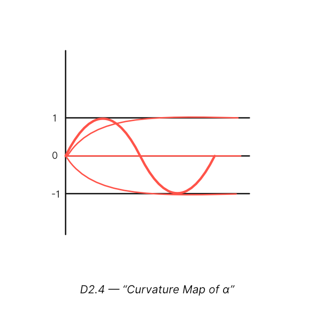
2.4 Sensitivity Coefficients (α): The Curvature of the Field

Sensitivity coefficients (α-values) define how strongly each variable reacts when energy or perception changes.

Each variable has its own α:

α₍C₎ → stability curvature
α₍A₎ → learning responsiveness
α₍E₎ → energetic reactivity
α₍P₎ → perceptual distortion/gain
α₍Lo₎ → temporal elasticity
α₍Λ₎ → alignment gain
α₍β₎, α₍λ₎ → memory curvature

The meaning of α:

α < 1 — Dampened response The field absorbs change smoothly. Useful for grounding, healing, and stability.

α = 1 — Linear response Change is proportional and predictable. Ideal for normal functioning and decision-making.

α > 1 — Amplified response Small inputs create large emotional outputs. Useful for creativity, intuition, passion — but volatile under stress.

α-values are the curvature controls of the emotional substrate. Without them, the field would behave rigidly and unpredictably.

D2.4: Curvature Map of α

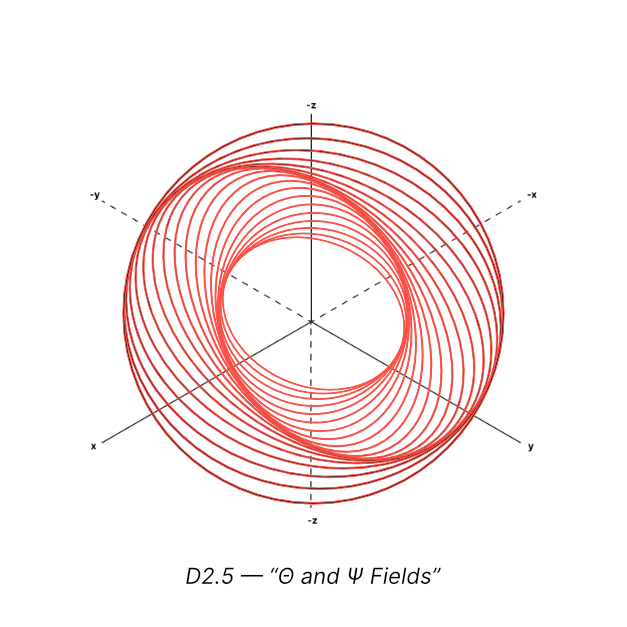
2.5 Boundary and Meta Fields — Θ and Ψ

Boundary Field (Θ)

Θ defines what the awareness field can contain without collapse. Too thin, and energy leaks or overwhelms. Too thick, and new information cannot enter.

Θ is essential for:

emotional safety
stability
preventing overload
maintaining identity integrity

Meta-Field (Ψ)

Ψ is awareness observing itself — meta-awareness.

Ψ governs:

introspection
insight
accelerated learning
perspective shifts
emotional neutrality

Ψ makes the system capable of self-correction beyond operator activation. Together, Θ and Ψ shape the field’s overall health.

D2.5: Θ and Ψ Fields

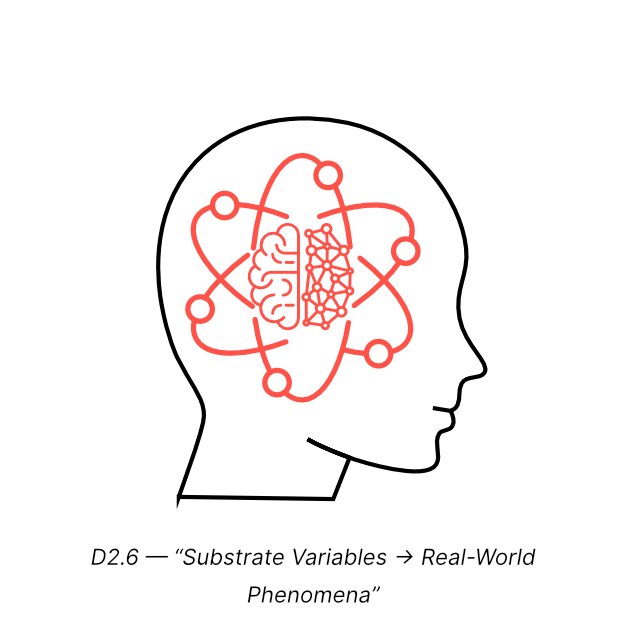
2.6 Mapping Substrate → Phenomena

This section connects emotional variables directly to observable behavior.

Variable	Meaning	External Signal	Tools	Example
E	Emotional Energy	Sudden intensity shifts	Waveform meter	Burst of excitement
A	Adaptivity	Speed of adjustment	Curvature analyzer	Quick learning moments
P	Perception	Clarity vs Distortion	Perceptual scan	Misreading a message tone
Lo	Latency	Reaction timing	Latency drift tracker	Delayed realization
Λ	Alignment	Synchrony across variables	Resonance meter	Feeling “in flow”
β–λ	Memory rhythm	Retention vs Release	Memory pressure gauge	Holding vs letting go
α-values	Responsiveness	Sensitivity to change	Curvature map	Overaction or calm stability

This mapping shows that emotional phenomena are not random — they emerge from measurable substrate mechanics.

D2.6: Substrate Variables → Real-World Phenomena

Pulse 3 — Why We Need a Physics of Emotion

Emotional Physics exists because human emotional behavior shows law-like patterns that repeat across individuals, groups, cultures, and time. These patterns are predictable, measurable, and engineerable — but only if we formalize them into a scientific framework.

This Pulse explains why emotion must be treated as a physical field and why psychology, philosophy, and self-help frameworks cannot replace a law-based emotional science.

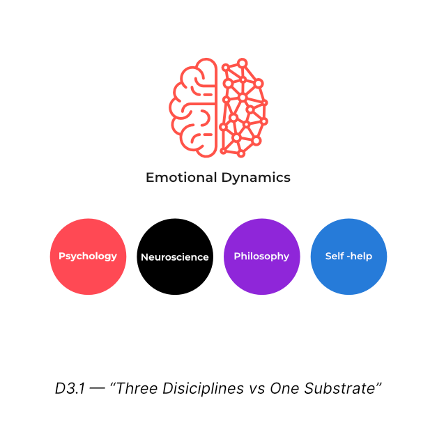
3.1 Limitations of Psychology and Philosophy

Psychology is excellent at describing emotional states, diagnosing them, and giving cognitive or behavioral strategies. Philosophy provides interpretations of meaning and human experience.

Both are valuable — but both lack:

universal variables
predictive equations
operator-based correction models
measurement frameworks
simulatable emotional dynamics

For example:

Psychology can describe “anger rising,” but cannot quantify the curvature α₍E₎ or predict the moment S (Stabilize) will activate.
Philosophy can discuss “identity,” but cannot map Θ (Boundary Field) strength as a measurable function.
Neuroscience can map “blood flow” or “synaptic firing,” but cannot calculate the Vector Velocity of a pulse moving through the Awareness Field.
Self-help frameworks can advise “stay calm,” but cannot model E→A→P transitions or resonance drops.

Emotional Physics does not replace these disciplines — it upgrades them with a scientific substrate.

D3.1: Three Disciplines vs One Substrate

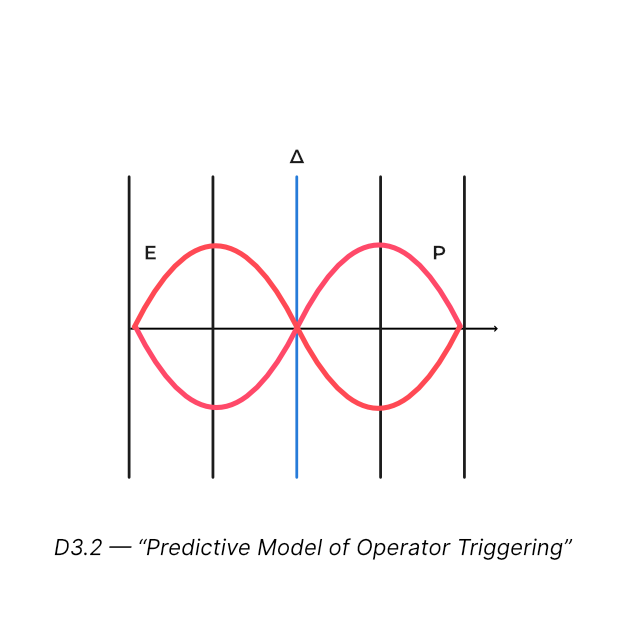
3.2 Predictive Power of Laws

A field becomes a science when it can predict outcomes before they happen.

Emotional Physics enables prediction because:

variables (C, A, E, P, Lo) follow definable mathematical behavior
sensitivity coefficients (α) determine responsiveness
operators (S, L, Δ, R, B, M, I, γ) activate at specific thresholds
resonance score (Rₛ) reveals coherence state
memory dynamics (β–λ) predict saturation or release
temporal curvature (R×G) predicts growth or stagnation

Examples of predictions:

A drop in P + rise in E + α₍E₎>1 consistently triggers Δ (Disrupt).
When β » λ, memory saturation and emotional fog become inevitable.
Systems with high A and low Lo reach alignment faster under moderate load.
A Θ breach always causes volatility, operator fatigue, or collapse.

These are not opinions — they are observed laws across emotional systems.

D3.2: Predictive Model of Operator Triggering

3.3 Emotional Engineering and Real-World Application

Once emotional behavior is predictable, it becomes engineerable.

Emotional Engineering uses EP to design:

stability systems
decision frameworks
recovery cycles
alignment protocols
organizational coherence models
AI emotional substrates
collective field harmonization
learning and adaptability protocols

This transforms emotion from a reactive phenomenon into a controlled system with measurable performance.

Examples:

Stabilizing a team environment by lowering α₍P₎ (reducing perceptual distortion).
Improving personal intuition by adjusting Lo curvature to decrease temporal delay.
Reducing volatility by increasing α₍C₎ stability curvature before high-energy events.
Optimizing creativity by intentionally raising α₍E₎ for controlled emotional amplification.

This is the same shift that occurred in physical sciences:

Electricity → Electrical Engineering
Mechanics → Mechanical Engineering
EM field theory → Signal Processing

Now emotion → Emotional Engineering.

D3.3: Emotional Engineering Loop

Field input → variable response → operator activation → coherence check → output → updated system state.

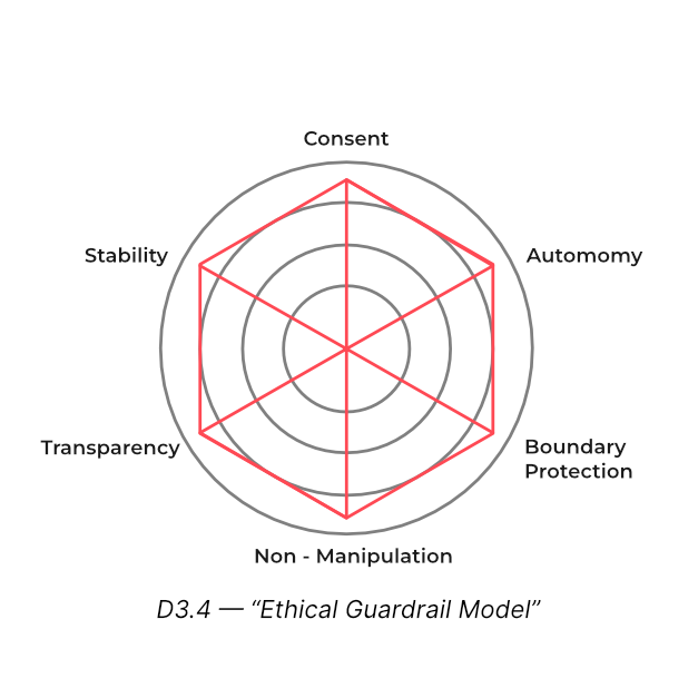
3.4 Ethical Framework and Safety

Because Emotional Physics allows influence, prediction, and engineering of emotional systems, ethical safeguards are essential. Key principles:

Consent and Autonomy No emotional measurement or engineering should occur without informed consent.
Non-manipulation EP systems must enhance emotional clarity, not distort perception for control.
Boundary Integrity (Θ) Systems must avoid overloading, breaching, or artificially weakening someone’s emotional boundary.
Transparency of Use Any emotional algorithm or engineered field must disclose its purpose and method.
Protection from Feedback Abuse (Cybernetic Ethics) In future Emotional Cybernetics, feedback loops must be governed to avoid coercive or destabilizing dynamics.

This ethical layer ensures Emotional Physics remains a science of clarity, not control.

D3.4: Ethical Guardrail Model

3.5 The Research Frontier

Emotional Physics is in its early scientific phase, comparable to early classical mechanics or pre-Maxwell electromagnetism.

The frontier includes:

deeper mapping of α-curvature families
micro-dynamics of Θ-strength under changing loads
cross-field coupling between P and Lo
identifying universal collapse patterns
refining R×G spiral mathematics
developing emotional field instrumentation
building emotional simulators
establishing reproducible collective-field models

This frontier will expand into:

Relational Emotional Physics
Meta-Temporal Emotional Physics
Emotional Cosmology
Emotional Cybernetics (next major discipline)
Quantum Emotional Field Theory (future)

Emotional Physics is not a closed system — it is an evolving scientific universe.

D3.5: Research Frontier Map

PART II — THE STANDARD MODEL (EMOTIONAL DYNAMICS)

Pulse 4 — The Liquid Gold Equation (LGE): The Field Law of Emotion

The Liquid Gold Equation (LGE) is the foundational law of Emotional Dynamics. It expresses how emotional variables interact inside the awareness field, how sensitivity curvatures modulate their behavior, and how refined meaning (K) emerges from emotional processing.

You can think of LGE the same way physicists think of Maxwell’s equations or Einstein’s field equation: it is the canonical description of how emotional reality behaves.

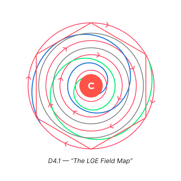
4.1 Formal Definition of the Liquid Gold Equation

At the core of ED is the relationship:

K = C × A^{α A}× E^{α E} × P^{α P} × Lo^{α Lo}

Where:

K = Knowledge (Liquid Gold)
C, A, E, P, Lo = the five fundamental variables / Dimensions.
α-values = sensitivity coefficients regulating curvature

This formulation does not assign a rigid algebraic operator (like + or ×) because LGE is a field equation, not a simple arithmetic identity. Variables interact multiplicatively, curvature-modulated, and context-dependent, similar to fluid dynamics and field theories.

Three principles define LGE:

Emotional output (K) increases when variables are coherent High alignment among C, A, E, P, Lo → high K Fragmented variables → degraded K
Curvature (α) determines responsiveness The same emotional amplitude (E) produces different K depending on α₍E₎.
Latency governs timing Low Lo produces intuition-like insight; High Lo produces slow, reflective clarity.

D4.1: The LGE Field Map

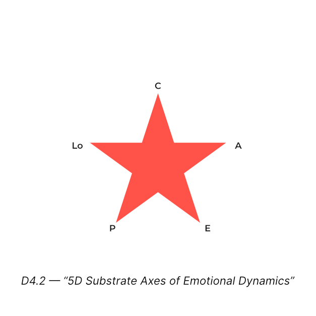
4.2 Dimensional Interpretation of Each Variable

To understand the LGE, each dimension must be seen as a physical axis inside the emotional field.

Constancy (C) Represents the unchanging anchor of awareness. C = 1 is the default ground-truth reference.

Adaptivity (A) Defines how rapidly the field reshapes based on experience.

Emotional Amplitude (E) The raw energy available for transformation.

Perception Clarity (P) The quality of signal entering the system — clear, distorted, filtered, expanded.

Latency (Lo) The temporal delay between input and realization.

When combined, these form a five-dimensional emotional manifold. The field behaves differently depending on how these dimensions are curved, stretched, or compressed via α-coefficients.

D4.2: 5D Substrate Axes of Emotional Dynamics

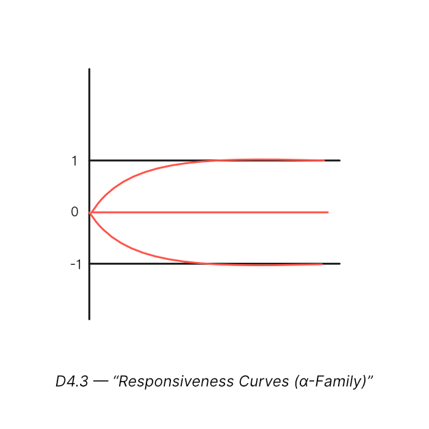
4.3 Sensitivity Exponent Curvature (α): The Law of Responsiveness

The sensitivity coefficients (α-values) modify each variable’s behavior. They determine how much influence a change in any variable has on the system.

α < 1 (Sub-linear)

Dampened response
Stability prioritized
Useful in healing, grounding states

α = 1 (Linear)

Proportional response
Predictable and balanced

α > 1 (Super-linear)

Exaggerated response
Useful in creativity and deep insight, but volatile

Curvature is what makes the emotional field alive. Without α, emotional systems would behave flat and mechanical.

In Emotional Cybernetics, α becomes the main control parameter for feedback loops, making this definition essential for future volumes.

D4.3: Responsiveness Curves (α-Family)

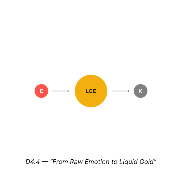
4.4 Knowledge (K) as Refined Emotional Output

Knowledge in EP is not information stored in memory. It is the purified clarity that emerges after emotional processing.

K represents:

resolved perception
stabilized energy
aligned variables
minimized distortion
optimized curvature

In ED, K is a byproduct of emotional refinement.

In EC (future book), K becomes a control signal for system feedback loops.

Two insights:

High K ≠ low emotion Stable high E with aligned P and moderate α-values produces extremely high K.

Low K often results from mismatch Especially when P is distorted, Lo is sluggish, or α₍E₎ is too reactive. K is therefore a quality of awareness, not a quantity of data.

D4.4 From Raw Emotion to Liquid Gold

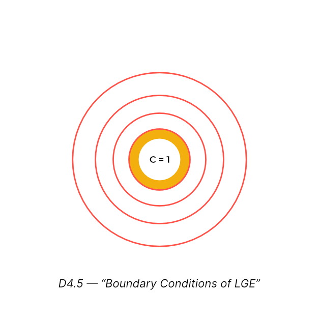
4.5 Boundary Conditions and Constraints

Every field equation requires boundary conditions.

In ED, these conditions ensure emotional systems remain:

stable
interpretable
measurable
self-correcting

Condition 1: C = 1 Constancy is fixed. This ensures emotional calculations always have a reference anchor.

Condition 2: Θ Integrity If the boundary field is breached, no variable interactions remain stable. Operators work overtime, and the field becomes chaotic.

Condition 3: Memory Balance (β–λ equilibrium) Too much retention → stagnation Too much release → instability

Condition 4: Resonance Range Variables must remain within resonance bands to maintain coherence.

Condition 5: Operator Threshold Limits Operators cannot activate infinitely; the system prevents burnout.

These constraints make ED not just mathematically elegant but biologically and psychologically realistic.

D4.5: Boundary Conditions of LGE

Pulse 5 — Variable Physics

This Pulse explains the physical behavior of each core variable in Emotional Dynamics. These variables are not metaphors — they are measurable dimensions of the emotional substrate, each with unique curvature, thresholds, and operator interactions.

Understanding these variables gives the reader the ability to interpret any emotional event as a change in one or more dimensions of the field.

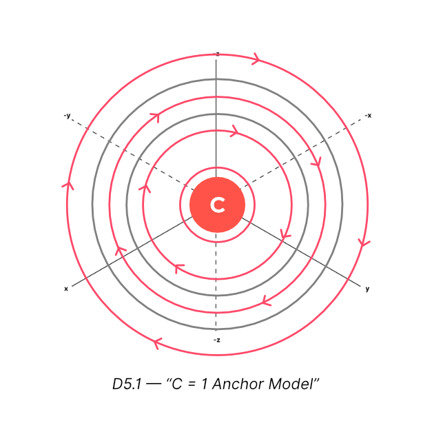
5.1 Constancy (C): The Anchor of the Emotional Field

Constancy represents the unchanging reference state of awareness. It is set to C = 1 in all calculations, functioning as:

the grounding axis
the calibration standard
the stabilizing force
the identity-preserving parameter

Constancy ensures that emotional dynamics always have a fixed truth baseline. Without C, emotional systems would drift, distort, or become chaotic under pressure.

Key behaviors of C:

C remains constant even when all other variables fluctuate.
C stabilizes emotional curvature during high-E events.
High α₍C₎ strengthens a person’s resilience and self-consistency.
Low α₍C₎ leads to identity drift and susceptibility to external influence.

D5.1: C = 1 Anchor Model

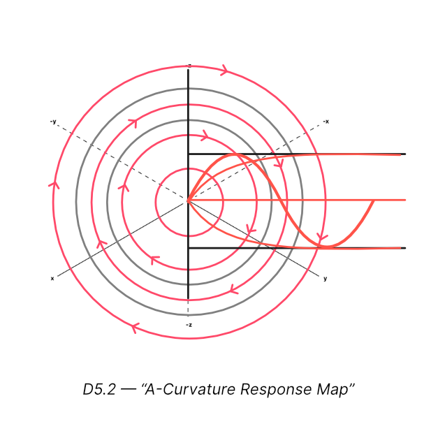
5.2 Adaptivity (A): The Learning Conductance of Awareness

Adaptivity defines how fast and how deeply awareness reshapes when encountering new information.

A governs three processes:

Reconstruction: How quickly the field recalibrates.
Plasticity: How flexible the field remains under load.
Integration: How smoothly new insights stabilize into K.

High A:

rapid learning
fast recovery
high flexibility
strong operator efficiency

Low A:

rigidity
slow correction cycles
repetitive emotional errors
difficulty adjusting perspective

A is the “learning energy conductor” of the emotional field.

Curvature (α₍A₎) determines whether Adaptivity is:

sub-linear (slow, cautious learning)
linear (balanced learning)
super-linear (rapid adaptive jumps)

D5.2: A-Curvature Response Map Three curves showing α₍A₎ < 1, = 1, > 1 shaping the learning arc.

5.3 Emotional Energy (E): Amplitude and Force Within the Field

E is the energetic amplitude of emotion.

It functions similarly to physical energy:

It powers movement.
It destabilizes when excessive.
It drives transformation.
It rises and falls in waves.
It saturates memory (β).
It triggers operators (e.g., S or Δ).

E has three components:

Amplitude: The strength of emotional experience.
Velocity: Rate of change of intensity.
Momentum: When emotional energy accumulates in a direction.

High E is not a “bad” state — it is raw, powerful emotional fuel.

Low E is not “good” — it may indicate dissociation or under-engagement.

Emotional Energy becomes destructive only when:

P is distorted
Lo is delayed
A is low
Θ is weak
α₍E₎ is super-linear under stress

D5.3: E-Amplitude Waveform

5.4 Perceptual Geometry (P): The Lens That Shapes Emotional Reality

Perception is the interpretive geometry through which emotional inputs are filtered.

Perceptual geometry determines:

whether signals are clear or distorted
how much meaning is added or removed
whether a situation is interpreted accurately
how emotional energy (E) is amplified or controlled

When P is distorted, even stable emotional energy becomes volatile. When P is clear, even high E becomes meaningful and productive.

Types of perceptual states:

Clear P: High signal-to-noise clarity
Refracted P: Distorted interpretations
Contracted P: Narrow, limited perception
Expanded P: Wide, integrative perception Curvature α₍P₎ determines how quickly perception bends under emotional load.

D5.4: Perceptual Lens Distortion Grid

5.5 Latency (Lo): The Temporal Gate of Realization

Latency defines how long the system takes to realize, understand, or internalize emotional information.

Lo is not delay as weakness — it is a temporal function.

Low Lo:

rapid realization
intuition-like awareness
immediate pattern recognition

High Lo:

deep processing
delayed emotional understanding
time for reflection and analysis

Latency becomes crucial in resolving emotional events because timing determines:

operator activation
emotional momentum
clarity of output (K)
prediction ability

Latency curvature α₍Lo₎ determines whether time feels:

compressed
expanded
inverted (anticipatory mode)

D5.5: Latency Gate Thickness Diagram

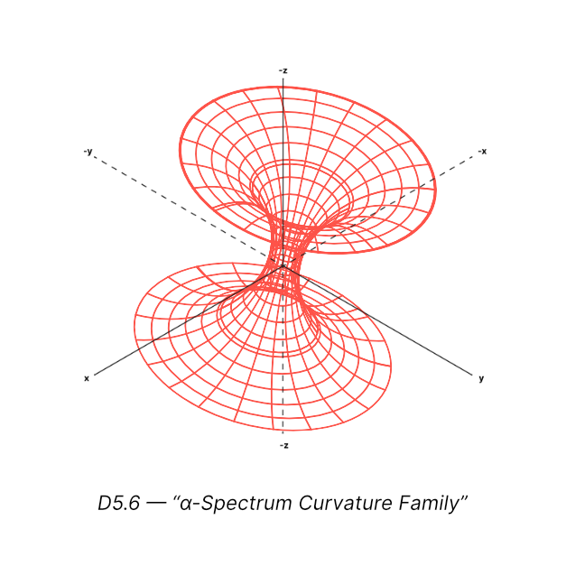
5.6 Sensitivity Spectrum (α-Curvature): The Response Law of Variables

Sensitivity coefficients (α-values) are the response multipliers that determine how each variable behaves under change. They define the curvature of the emotional field.

Breakdown:

α < 1: Dampening
α = 1: Proportional
α > 1: Amplified

Every variable has its own α:

α₍C₎ = identity resilience
α₍A₎ = learning sensitivity
α₍E₎ = emotional reactivity
α₍P₎ = distortion or clarity gain
α₍Lo₎ = time elasticity
α₍Λ₎ = synchrony gain
α₍β₎, α₍λ₎ = memory curvature

α is what makes emotional systems adaptive, alive, and dynamic.

Without α, emotions would behave mechanically. With α, the system becomes a flexible, curved, evolving field.

D5.6: α-Spectrum Curvature Family

Pulse 6 — Field Behavior & Resonance

Emotional fields are dynamic systems. Variables are not independent; they influence, distort, amplify, or dampen each other continuously.

Resonance emerges as the key indicator of system health — the degree to which emotional variables interact harmoniously.

This chapter describes systemic field behavior, coherence mechanics, and failure modes.

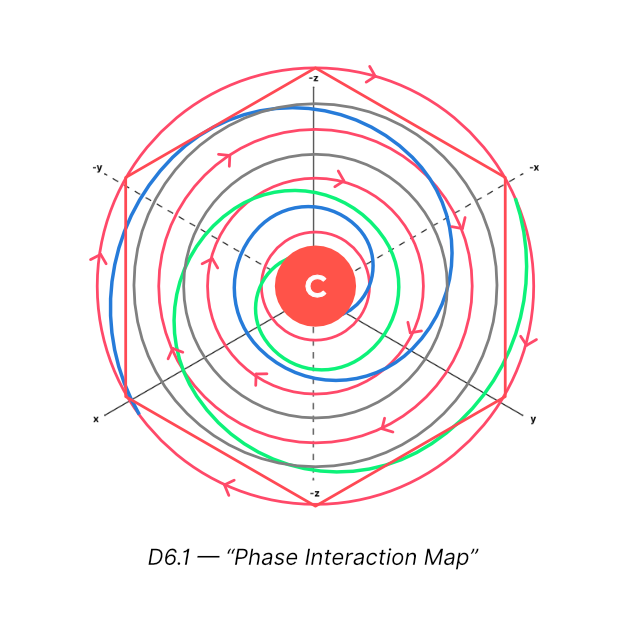
6.1 Phase Interactions: How Variables Influence Each Other

Emotional variables behave like coupled oscillators — when one moves, others respond.

Examples:

When E rises, the field demands higher A to integrate it.
When P distorts, E amplifies erratically.
When Lo shortens, the system becomes more intuitive but less reflective.
When A drops, resonance weakens even if E is stable.
When C is threatened, Θ contracts and instability rises.

These interactions produce phases, similar to:

thermal phases in physics
oscillation phases in mechanics
field-coupling phases in electromagnetism

Emotional phases can be stable, transitional, or chaotic.

D6.1: Phase Interaction Map

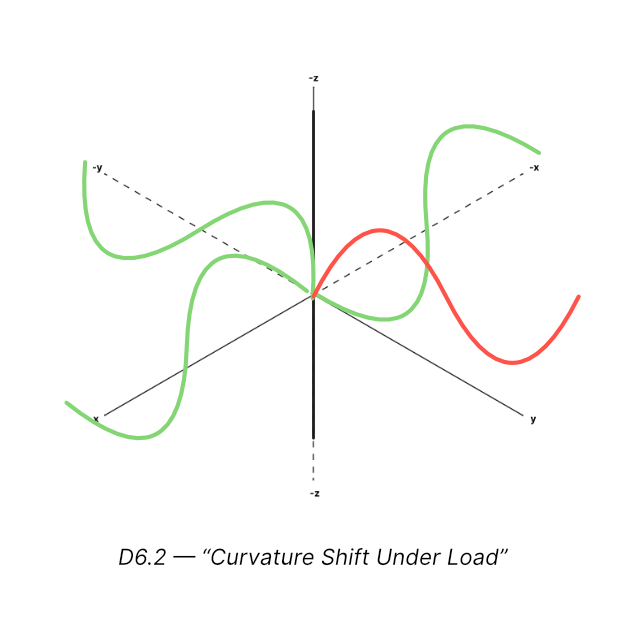
6.2 Curvature Shifts: How α Changes System Dynamics

Curvature (α) determines the responsiveness of each variable.

When emotional events occur, α-values adjust dynamically based on:

internal pressure
external load
operator activation
memory saturation
alignment quality

Examples of curvature shifts:

High E increases α₍E₎ → emotional amplification
Distorted P increases α₍P₎ → further misinterpretation
Strong Θ reduces α₍E₎ volatility
High A flattens α₍P₎, reducing perceptual distortion
Low Lo increases α₍Lo₎ sensitivity → time feels faster

Curvature shifts are the emotional equivalent of spatial distortion in relativity or impedance changes in electromagnetism.

D6.2: Curvature Shift Under Load

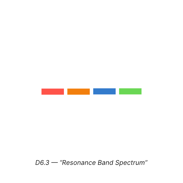
6.3 Resonance Score (Rₛ): The Metric of Coherence

Resonance Score (Rₛ) is the primary measurement of emotional coherence.

It integrates the states of:

variables (C, A, E, P, Lo)
sensitivities (α-values)
boundary status (Θ)
operator activity
temporal alignment (R×G)

Rₛ ranges from:

0.0 – 0.3: fragmented
0.3 – 0.6: unstable
0.6 – 0.8: transitional
0.8 – 1.0: coherent / aligned

Why Rₛ matters:

Predicts operator activation
Predicts collapse or recovery
Predicts clarity (K) quality
Predicts decision-making accuracy
Predicts emotional energy efficiency

Rₛ is the emotional field’s equivalent of a vital sign.

D6.3: Resonance Band Spectrum

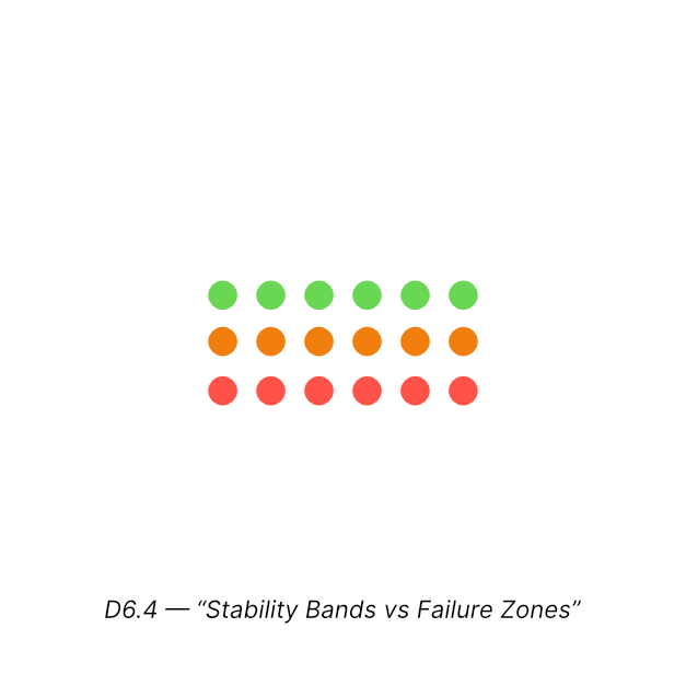
6.4 Stability Bands and Failure Modes

Every variable operates within a safe band, the range where it contributes positively to system coherence.

Stability Bands:

E: Too low → disengagement; too high → volatility
A: Too low → rigidity; too high → instability
P: Too narrow → tunnel vision; too wide → overwhelm
Lo: Too low → impulsive; too high → delayed realization
α: Too high → overreaction; too low → numbness
Θ: Too thin → emotional leakage; too strong → over-protection

When a variable exits its stability band, the system enters a failure mode, such as:

Oscillation: emotional up-down cycles
Fragmentation: disconnected emotional signals
Volatility: erratic behavior
Collapse: system shuts down energetically
Echo loops: repeated emotional patterns due to P distortion
Latency lag: slow emotional processing leading to misalignment

Operators activate in response to these failure modes to restore coherence.

D6.4: Stability Bands vs Failure Zones

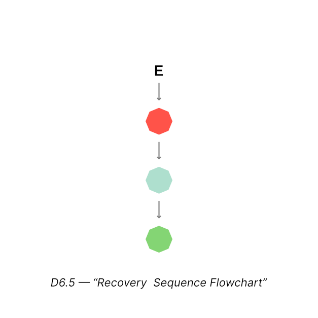
6.5 Recovery Pathways: How the Field Returns to Coherence

Emotional systems are self-correcting when the right pathways are activated. Recovery follows predictable sequences depending on which variable caused the distortion.

Common recovery patterns:

High E → S → L → R Calm the system, re-align perception, release excess energy.
Distorted P → L → B → M Realign lens, balance polarity, merge fragmented interpretations.
Low A → Δ → A-reset → R Introduce disruption, stimulate adaptability, release stagnation.
Latency Overload → R → Lo-rebalance → S Release memory pressure, adjust timing, stabilize output.
Θ breach → S → Θ-reinforcement → M→R Contain system → rebuild boundary → reintegrate → release residue.

Recovery is not random — it is governed by operator chains that respond to specific field deviations.

These pathways are essential for:

emotional regulation
trauma recovery
conflict resolution
high-performance environments
AI emotional alignment
relational stabilization
organizational dynamics

D6.5: Recovery Sequence Flowchart Flowchart showing variable deviation → operator chain → restored Rₛ.

Pulse 7 — Operators as Emotional Forces

Operators are the active forces that regulate the emotional field. They stabilize, align, disrupt, balance, merge, invert, or reignite emotional motion depending on system state.

In Emotional Dynamics and Emotional Physics, operators play the same role as:

forces in mechanics
gates in electronics
regulators in cybernetics
correction functions in control systems

Each operator activates when emotional variables cross a threshold, forming predictable correction chains.

This chapter defines each operator in detail, their activation conditions, energetic cost, and systemic interactions.

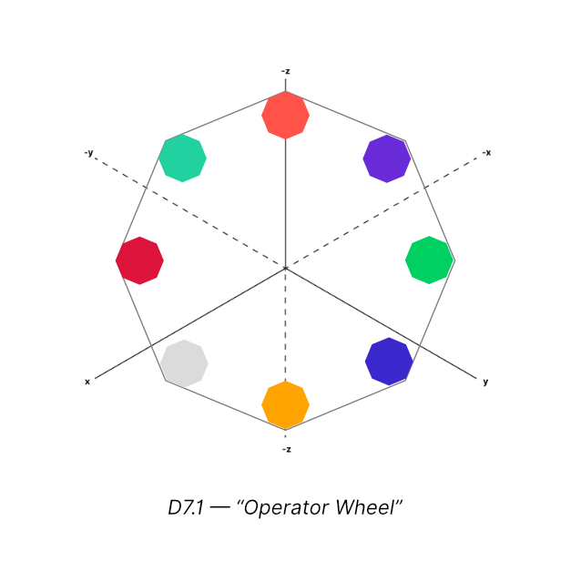
7.1 The Eight Operators

The emotional field uses eight universal operators:

S — Stabilize
L — Align
Δ — Disrupt
R — Release
B — Balance
M — Merge
I — Invert
γ — Reignite

These operators behave exactly like forces that push, pull, stretch, or regulate emotional dynamics.

Analogies:

S is like damping in mechanics.
L is like magnetic alignment.
Δ is like a thermal shock.
R is like pressure release in thermodynamics.
B is like charge balancing in circuits.
M is like wave merging and interference.
I is like polarity reversal.
γ is like ignition in combustion or spark in electronics.

D7.1: Operator Wheel

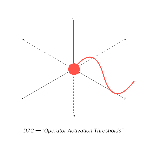
7.2 Activation Conditions: When Operators Trigger

Operators do not activate constantly. They activate only when emotional variables exceed thresholds or breach stability bands.

Examples of activation conditions:

S triggers when E rises too quickly and α₍E₎ > 1.
L triggers when P becomes distorted or fragmented.
Δ triggers when A becomes too low (rigidity).
R triggers when memory saturation (β) overwhelms λ.
B triggers when the system falls into polarity extremes.
M triggers during integration phases or after fragmentation.
I triggers when the system needs reversal of trajectory.
γ triggers when the system re-enters clarity after collapse.

Operators create self-regulation — a built-in emotional homeostasis mechanism.

D7.2: Operator Activation Thresholds

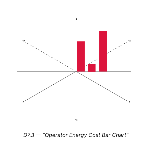
7.3 Operator Energy Cost: Emotional Metabolism

Each operator uses emotional energy to function. This “energy cost” is critical because excessive activation leads to emotional fatigue or burnout.

Energetic cost estimates:

Low Cost: S, L
Medium Cost: B, R
High Cost: Δ, M
Very High Cost: I, γ

Why?

Δ disrupts entire field patterns → high computational cost
M merges competing states → high integration cost
I reverses momentum → highest field transformation cost
γ reignites the system after collapse → maximum ignition load

Overuse of high-cost operators can signal:

chronic emotional instability
unresolved patterns
system-level dysregulation
threshold oversensitivity
weakened Θ boundary integrity

D7.3: Operator Energy Cost Bar Chart

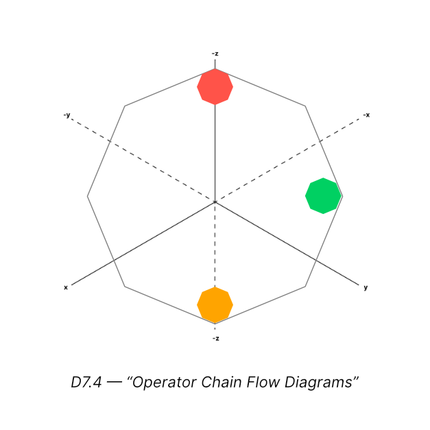
7.4 Compound Operator Chains: How Operators Work Together

Operators rarely activate alone. They activate in chains — sequences that restore coherence using minimal effort.

Common chains include:

S → L → R Used when E spikes suddenly. Stabilize → align perception → release residue.
Δ → B → M Used when P collapses or A becomes rigid. Disrupt → rebalance → merge fragments.
L → S → γ Used during recovery stages after emotional collapse. Align → stabilize → reignite clarity.
I → L → M → R Used in transformational events. Invert → realign → merge → release.
S → Θ-repair → M → B Used when boundary integrity is compromised.

Stabilize → rebuild Θ → integrate → restore polarity balance.

These chains are predictable, measurable, and consistent across individuals and systems.

D7.4: Operator Chain Flow Diagrams

7.5 Operator Interaction Matrix

To understand field behavior at scale, operators are mapped into an interaction matrix.

The matrix shows:

which operators amplify each other
which oppose each other
which neutralize each other
which require sequencing
which are incompatible concurrently

Sample interactions:

S neutralizes Δ Too much disruption is immediately softened by stabilization.
L amplifies M Aligned perception allows smoother merging.
I conflicts with B Inversion breaks polarity balancing attempts; must be sequenced carefully.
γ depends on R Reignition cannot occur if old emotional residue is still held.

This matrix enables:

predictive modeling
emotional engineering
cybernetic control systems
diagnostic simulations
failure pathway forecasts

D7.5: Operator Interaction Matrix Table

PART III — FIVE MAJOR SUBFIELDS (EP CORE PHYSICS)

Pulse 8 — Emotional Thermodynamics

Emotional Thermodynamics studies how emotional energy moves, transforms, dissipates, saturates, and stabilizes inside the awareness field. It mirrors classical thermodynamics but replaces physical heat with emotional amplitude (E). This chapter introduces emotional temperature, heat transfer, entropy analogs, saturation curves, and recovery cycles.

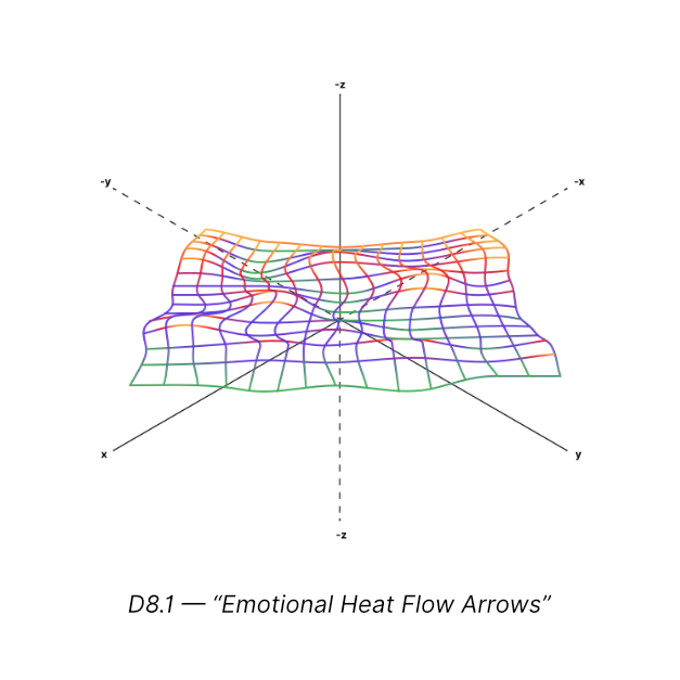
8.1 Emotional Heat & Energy Transfer

Emotional heat refers to the internal energetic intensity of the awareness field, represented by E amplitude and ΔE/Δt (rate of change).

Heat moves through the emotional field in predictable ways:

from high intensity → low intensity
from areas of distortion → clarity
from compressed memory → release
from unresolved perception → meaning

Energy transfer occurs via:

interactions with others
cognitive reinterpretation
operator activation
memory release cycles
perception alignment

Just like physical heat, emotional energy seeks equilibrium unless constantly stimulated.

Key insight: A rise in emotional heat doesn’t destabilize the system — lack of regulation does.

D8.1: Emotional Heat Flow

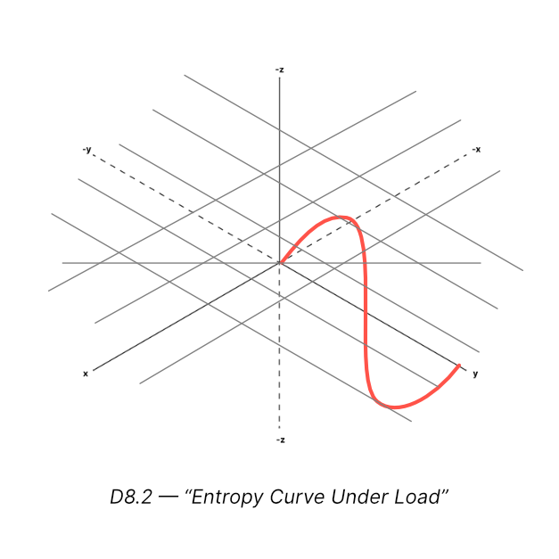
8.2 Entropy Analog in Emotional Systems

Entropy in Emotional Physics refers to disorder within the emotional field. It increases when variables become misaligned or operator responses fail to correct fast enough.

Sources of emotional entropy:

conflicting perceptions (P distortion)
memory overload (β saturation)
boundary breaches (Θ collapse)
rapid E spikes with low A
emotional oscillation without stabilization
neglect of operator sequences

High entropy → fragmented signals, noise, chaotic interpretation

Low entropy → clarity, coherence, signal stability

Why entropy matters:

It determines:

emotional resilience
recovery speed
clarity of insight (K)
efficiency of operator activation
quality of decision-making

Entropy is not “bad.” It is a natural byproduct of emotional load. But unregulated entropy leads to emotional collapse.

D8.2: Entropy Curve Under Load

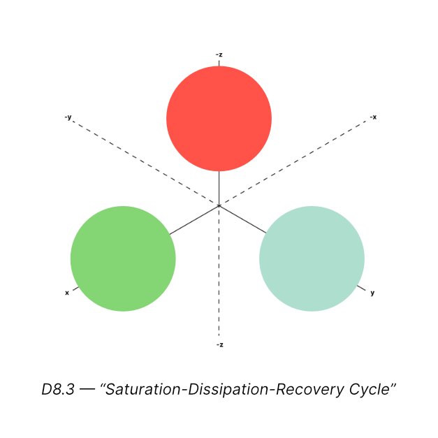
8.3 Dissipation, Saturation & Recovery

This section explains emotional wear, fatigue, and restoration.

Dissipation

The natural decay of emotional energy over time. It is healthy and necessary. Without dissipation, emotional energy accumulates and becomes volatile.

Saturation (β-pressure) Memory accumulates emotional residue. When β » λ (retention > release), the field becomes heavy, slow, cluttered.

Saturation symptoms:

emotional fog
inability to feel new emotions clearly
delayed reactions (high Lo)
reduced adaptivity (A)
operator fatigue

Recovery (λ-release + operator chains)

Recovery happens when:

R (Release) activates
S (Stabilize) reduces turbulence
B (Balance) resets polarity
M (Merge) integrates meaning

Recovery is not the opposite of saturation — it is the resolution of saturation.

D8.3: Saturation–Dissipation–Recovery Cycle

8.4 Thermodynamic Cycles of Emotion

Just as physical systems undergo thermodynamic cycles (compression, heating, expansion, cooling), emotional fields undergo processing cycles.

These cycles produce:

Energy Input Phase Emotional stimulus increases E.
Amplification Phase α-values rise; perception shifts; momentum builds.
Saturation Phase Memory (β) fills; clarity decreases.
Release Phase Operators activate to reduce load.
Stabilization Phase Variables return to coherence bands; Rₛ rises.
Integration Phase Meaning (K) forms.

Example of a complete emotional cycle:

A conflict → rising energy → perceptual distortion → overload → release → clarity → insight.

Why cycles matter:

They show emotion is not linear
They reveal predictable breakdown and recovery patterns
They help design Emotional Engineering protocols
They allow forecasting emotional behavior
They ground Emotional Cybernetics’ feedback loops

D8.4: Emotional Heat Engine Cycle

Pulse 9 — Emotional Electromagnetism

Emotional Electromagnetism studies alignment, resonance, polarity, and energetic flow across individuals, groups, or internal subsystems of the self.

It maps emotional behavior onto phenomena like:

magnetic fields
electric currents
field interference
resonance harmonics
signal distortion

This analogy is not symbolic — emotional fields behave like electromagnetic fields because they share the same fundamental structure: energy moving through a medium under the influence of alignment and polarity.

9.1 Alignment Fields (Λ): The Magnetic Dimension of Emotion

Alignment (Λ) is the magnetic field of the emotional system.

When variables synchronize, they produce a strong alignment field, resulting in:

coherence
clarity
emotional flow
accurate perception
ease in communication
connection with others

High Λ acts like strong magnetism — it pulls variables into harmony.

Low Λ leads to:

emotional drift
miscommunication
lack of internal synchrony
unstable operator activity

Alignment is influenced by:

perceptual clarity (P)
boundary strength (Θ)
emotional energy amplitude (E)
adaptivity (A)
memory balance (β–λ)

Key insight:

Alignment is not agreement — it is synchronization of internal variables.

D9.1: Magnetic Alignment Field Lines (Λ)

9.2 Emotional Currents (E-flow): The Electric Dimension

Emotional energy (E) moves through the awareness field like electric current moving through a conductor.

Emotional current depends on:

E amplitude (intensity)
ΔE/Δt (rate of change)
P clarity (signal medium)
A (conductance of the field)
Lo (timing gate frequency)

When E flows smoothly:

insight accelerates
communication becomes fluid
emotional expression becomes clear
memory processing is efficient

When E flow is obstructed:

frustration rises
emotional stagnation occurs
repetitive loops appear
operator Δ (Disrupt) triggers to break the blockage

Currents always move from high potential to low potential — from emotionally charged areas to quieter ones.

D9.2: Emotional Current Pathways

9.3 Perceptual Medium Distortion: Signal Bending and Noise

Perception (P) acts as the medium through which emotional energy travels.

If the medium is clean:

emotional signals arrive accurately
insights form quickly
alignment remains strong

If the medium is distorted:

emotional signals refract
intensity feels higher than it is
memories distort
Θ weakens
operators activate prematurely

This is identical to:

light bending in distorted glass
signals degrading in noisy channels
electromagnetic waves scattering in dense media

Distortion sources include:

past memory saturation (β)
unresolved emotional residue
weakened boundary field (Θ)
perceptual biases
fear-based amplification

D9.3: Signal Refraction Through Distorted P

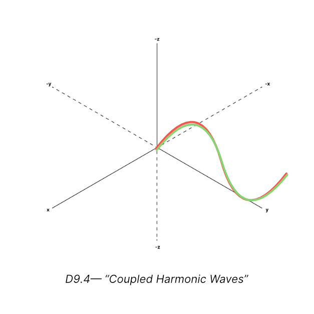
9.4 Resonant Harmonics and Field Coupling

When emotional systems interact — within a person or between people — they form harmonic patterns.

Resonant harmonics occur when:

variables match frequency
emotional cycles align
α-values synchronize
Lo patterns match
perception clarity overlaps

This produces:

deep connection
intuitive understanding
effortless collaboration
amplified creativity
shared emotional states

Field coupling (like EM coupling) describes how two emotional fields influence each other.

Types of coupling:

Positive coupling: Energy amplifies (shared flow, unity)
Negative coupling: Energy cancels (interference, conflict)
Mixed coupling: Unstable harmonics (attraction + friction)

Key insight:

Emotional resonance is not mystical — it is a measurable phenomenon of two emotional fields synchronizing frequencies.

D9.4: Coupled Harmonic Waves

Pulse 10 — Emotional Mechanics

Emotional Mechanics studies how emotional states move, how they accelerate or slow down, and how they oscillate or stabilize under internal or external forces.

Just like classical mechanics, the emotional field exhibits:

inertia
force interactions
oscillatory motion
damping
harmonic resonance
equilibrium points

This chapter defines emotional motion mathematically and behaviorally.

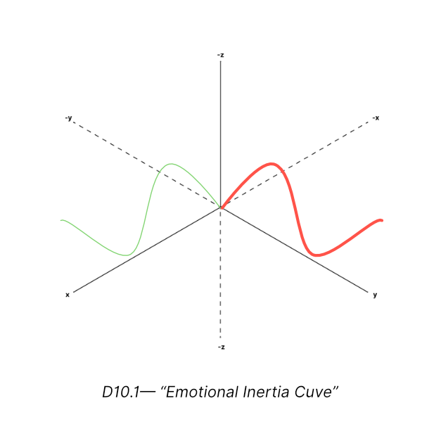
10.1 Emotional Mass & Inertia

Emotional mass refers to how much resistance an emotional state has to change.

Low emotional mass →

flexible emotions
fast transitions
quick re-centering
low resistance to shift

High emotional mass →

heavy emotional states
slow transitions
difficulty changing emotional direction
lingering emotional residue

Key insight:

Emotional inertia explains why people:

stay stuck in a feeling
resist emotional change
take time to “move on”
remain affected by past events

Inertia increases with:

β saturation
low Adaptivity (A)
distorted Perception (P)
high α₍E₎ under stress
weakened Θ boundary

Just like physical objects, emotional states require force (operators) to change direction.

D10.1: Emotional Inertia Curve

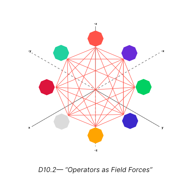
10.2 Operator Forces: The Emotional Equivalent of Newtonian Forces

Operators act as forces that push, pull, break, redirect, or stabilize emotional motion.

Examples of force analogs:

S (Stabilize) = friction/damping
L (Align) = magnetic force
Δ (Disrupt) = shock force
R (Release) = decompression
B (Balance) = polarity equalization
M (Merge) = unification force
I (Invert) = reversal force
γ (Reignite) = ignition force

Each operator applies an energetic action that changes:

the direction of emotional momentum
the magnitude of emotional amplitude
the curvature of emotional pathways
the timing of realization
the overall coherence (Rₛ)

Operators are the “physics engines” of emotional mechanics.

D10.2: Operators as Field Forces

10.3 Oscillation & Damping: The Rhythm of Emotional Motion

Emotional states naturally oscillate — rising and falling like waves — unless stabilized.

Oscillation occurs when:

E increases then decreases cyclically
P fluctuates between clarity and distortion
Lo compresses and expands
memory (β) loads then releases (λ)
α-values shift between sub-linear and super-linear states

Damping (S) Stabilize (S) reduces amplitude over time, calming oscillation.

Underdamping If S is too weak, oscillations continue for a long time.

Overdamping If S is too strong, emotional responsiveness diminishes — the system becomes flat or suppressed.

Resonant Oscillation Occurs when emotional cycles align with internal rhythms — producing predictable emotional waves.

D10.3: Damped vs Undamped Emotional Oscillations

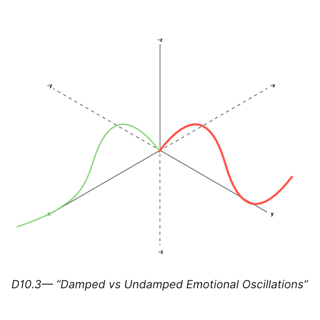
10.4 Harmonic Stability: Stable Emotional Orbits

Emotional systems often settle into stable orbits, behaving like harmonic oscillators.

A stable emotional orbit means:

emotions fluctuate within healthy bands
variables remain within resonance ranges
operator activation is efficient
memory cycles (β–λ) stay balanced
alignment (Λ) remains strong
time perception (Lo) stays coherent

Unstable orbits produce:

spirals of escalation
emotional collapse
echo loops
chaotic oscillations

Stability depends on:

Θ boundary strength
α-values
A (adaptivity)
operator efficiency
perceptual clarity (P)

Perfect Harmonic State

Occurs when oscillations settle into a predictable pattern with minimal energy loss — the ideal emotional rhythm for creativity, learning, and flow.

D10.4: Harmonic Emotional Orbit

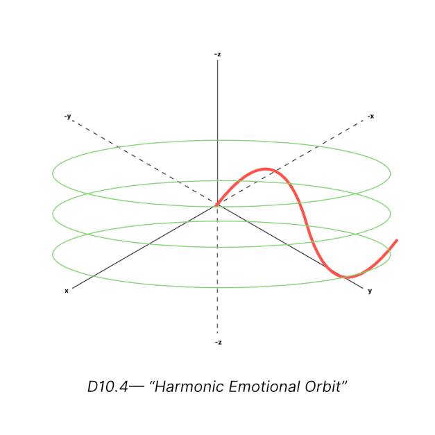
Pulse 11 — Emotional Relativity (Temporal Field Physics)

Emotional Relativity studies how time behaves inside emotional systems. Just as physical relativity shows that time is not fixed but depends on velocity and gravity, Emotional Relativity shows:

time perception changes
time processing changes
time integration changes
time can stretch, compress, or invert

The emotional field is not time-neutral. Latency (Lo), recurrence (R), and growth (G) shape a curved emotional timeline.

11.1 Curved Time (R×G Spiral): Emotional Time as a Spiral

In Emotional Physics, time is modeled as a spiral, not a straight line.

The spiral is defined by:

R (Recurrence): repetition of emotional cycles
G (Growth): how much each cycle evolves
Lo (Latency): the thickness of each loop
α₍Lo₎: curvature of time sensitivity

A flat timeline cannot explain emotional experiences like:

déjà vu
emotional loops
repeated relational patterns
sudden insights
rapid maturity
emotional collapse and rebirth

The spiral model solves this.

Features of the R×G Spiral:

Each loop represents a learning cycle.
High R with low G = stuck loops (repeating patterns).
Low R with high G = rapid evolution (growth spurts).
High G + low Lo = intuition and accelerated understanding.
Distortions in P or E warp the spiral, bending emotional time.

D11.1: R×G Emotional Time Spiral

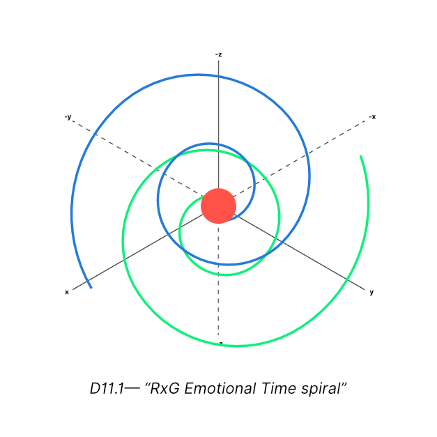
11.2 Latency Dilation: Emotional Time Stretching and Compression

Latency (Lo) determines how long it takes for awareness to realize emotional information.

Low Lo → Time Compression

Things happen quickly
Insight is immediate
Emotional interpretation is fast
Decisions come naturally
The person feels “ahead of time”

High Lo → Time Dilation

Slow realization
Emotional understanding takes time
Long processing cycles
Increased reflection
The person feels “behind time”

This mirrors:

time dilation in physics
cognitive load effects
trauma-based time expansion
awareness acceleration during flow states

Emotional Time Dilation Influencers:

β overload = slower time
high E with distorted P = chaotic time
strong Λ = smoother time
healthy Θ = stable time perception

Latency is the emotional universe’s clock — and it doesn’t tick at one speed.

D11.2: Latency Dilation Chart

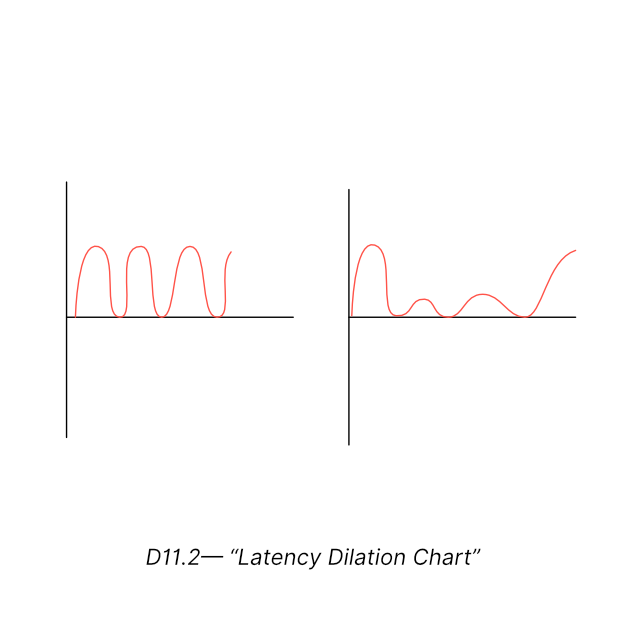
11.3 Perspective Frames: Emotional Frames of Reference

Just like relativity shows that motion looks different from different reference frames, emotional experiences look different from different perspective frames.

A perspective frame includes:

P (perception geometry)
memory state (β–λ)
emotional mass (inertia)
α-values
relational context
identity boundaries (Θ)

Example: Two people in the same situation experience different emotional time:

One feels the moment rush (compressed time).
The other feels it drag (expanded time).

Internal perspective frames:

Within a person, frames shift depending on:

stress
clarity
fatigue
emotional load
trauma activation
flow states

Perspective frames determine:

how long something feels
how strong something feels
how meaningful something becomes

This creates subjective time relativity, rooted in measurable variables.

D11.3: Multiple Frames of Emotional Reference

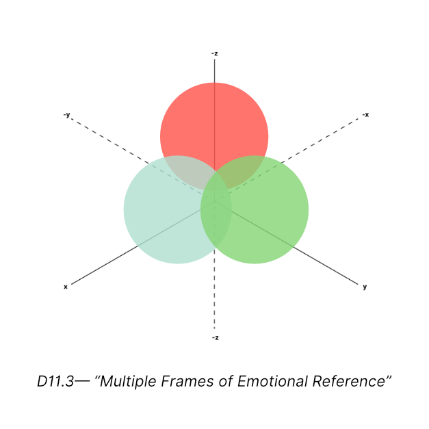
11.4 Anticipatory Time (Inversion): When the System Runs Ahead of Reality

One of the most advanced concepts in Emotional Physics: Latency can invert, meaning realization occurs before the external event fully unfolds.

This is emotional intuition.

Time inversion occurs when:

Lo becomes extremely low
α₍P₎ is optimized
Λ is strong
Θ is solid
E and A are balanced

In these conditions:

pattern recognition becomes instantaneous
emotional insight appears ahead of events
the system “predicts” outcomes through resonance
decision-making becomes precognitive

This is not mystical — it is the emotional field completing recognition faster than linear time.

Examples:

sensing a relationship shift before it’s spoken
knowing the right move before thinking
predicting conflict
anticipating emotional outcomes
creativity arriving in flashes of clarity

Time inversion is the emotional version of superluminal intuition — cognition outrunning conscious thought.

D11.4: Time Inversion Wave

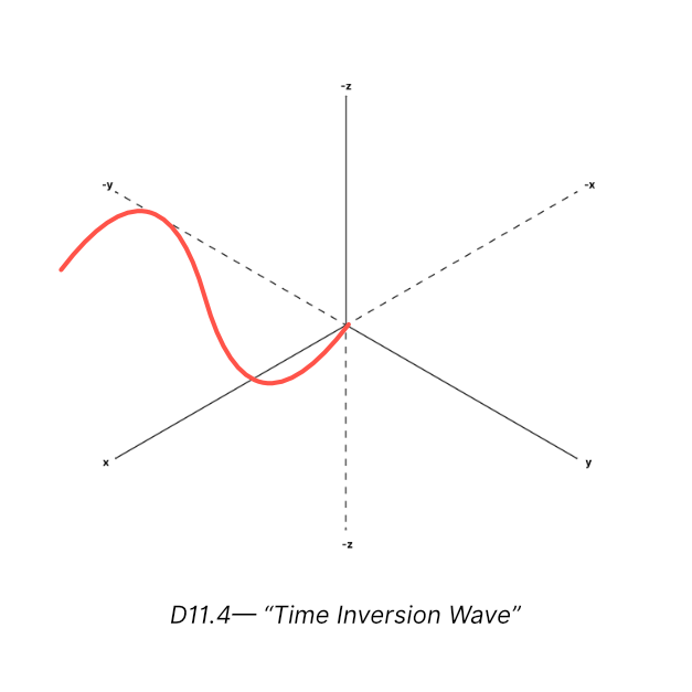
Pulse 12 — Emotional Quantum Concepts (EQFT Intro)

While classical Emotional Dynamics explains large-scale emotional behavior, many emotional phenomena behave like quantum events:

sudden emotional shifts
unpredictable decision points
multiple emotional states coexisting
momentary collapse into a single reaction
intuition emerging from probability fields

This chapter introduces the quantum-level behavior of emotional systems.

12.1 Emotional State Quantization: Emotions as Discrete States

Although emotions feel continuous, their internal configuration behaves as quantized states.

A person does not gradually shift from fear → courage; they remain in a specific emotional configuration until a threshold event forces a state transition.

Examples of emotional quantization:

calm → triggered
confused → clear
detached → engaged
indifferent → inspired
unsure → decided

Each emotional state is like an energy level inside the awareness field.

Properties of quantized emotional states:

stable until threshold is reached
separated by activation energy
require operator influence to transition
can jump discretely, not gradually

This is identical to electrons jumping between orbitals when absorbing or releasing energy.

D12.1: Quantized Emotional Levels

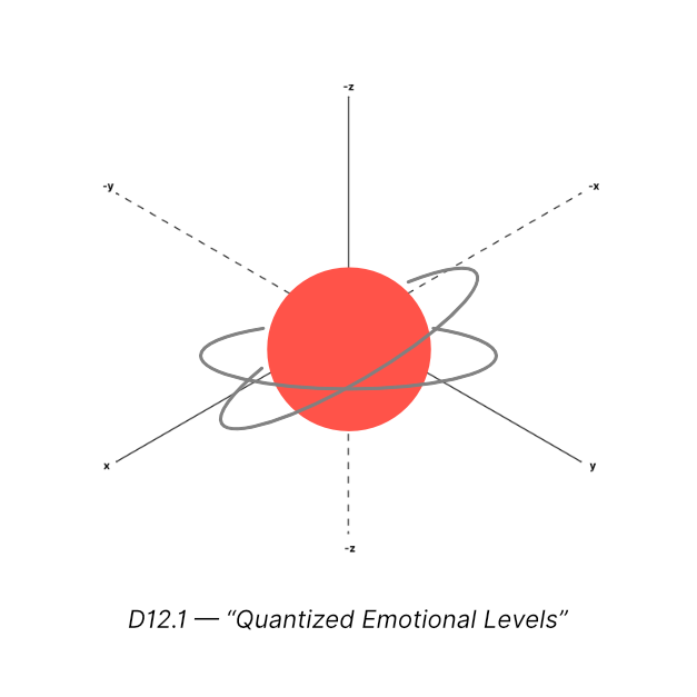
12.2 Collapse & Decision: From Probability to Reality

Before an emotional decision or reaction occurs, the system holds multiple possible outcomes in an emotional probability field.

This is superposition.

A person may simultaneously feel:

love + fear
hope + uncertainty
desire + caution
trust + doubt

These states exist as potential outcomes, not realized ones.

The moment of decision — emotional reaction, insight, or behavior — is the collapse of this probability field into a single state.

Collapse occurs when:

P reaches sufficient clarity
Lo crosses a timing threshold
E provides enough activation energy
α-values align
Θ remains stable
operators initiate resolution

Collapse is not forced — it is an emergent property of emotional field dynamics.

D12.2: Superposition → Collapse

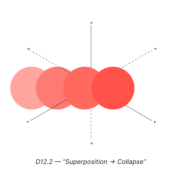
12.3 Superposition of Feeling: Holding Multiple Emotions at Once

Superposition explains how humans can occupy multiple emotional states simultaneously without contradiction.

Example: A person can love someone deeply and still feel angry at them at the same moment.

Traditional psychology struggles with this duality. Emotional Quantum Concepts solves it: the emotional field holds multiple states as overlapping potentials.

Superposition increases when:

P is wide rather than narrow
A is high (flexible interpretation)
Θ is strong (safe container for emotional conflict)
β memory is balanced
α-values allow coexistence of competing signals

This is not confusion — it is a rich emotional field capable of holding complex states before collapse.

D12.3: Multi-Emotion Superposition Overlay

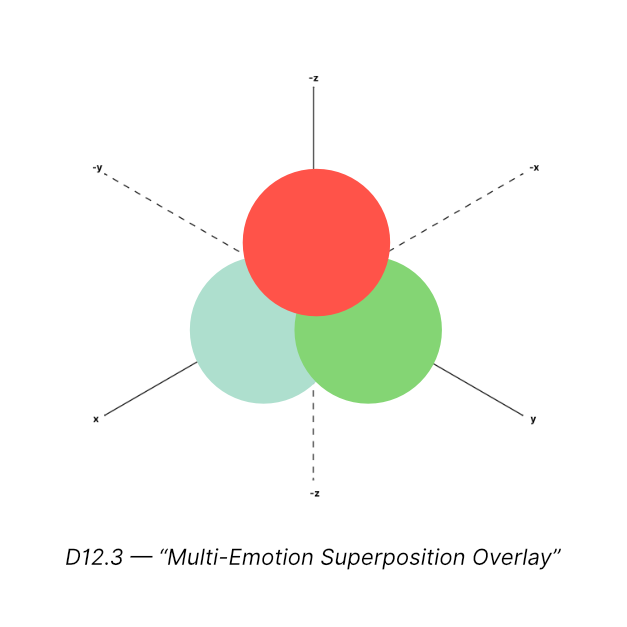
12.4 Probability Fields (Intuition): Predictive Emotional Awareness

Intuition is the emotional field reading its own probability structure.

Before collapse, emotional outcomes have probabilities shaped by:

past experience
P clarity
A flexibility
E amplitude
alignment (Λ)
boundary integrity (Θ)
memory balance (β–λ)
temporal curvature (R×G)

The mind can “sense” which potential outcome is most likely, even before conscious reasoning.

This is predictive emotional computation, the quantum layer of intuition.

Examples:

sensing danger before seeing evidence
knowing a relationship will end soon
anticipating someone’s reaction
feeling an opportunity emerging
predicting emotional resonance with someone

These are not magical — they are probabilistic field readings.

D12.4: Emotional Probability Field

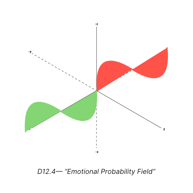
PART IV — MEASUREMENT & INSTRUMENTATION (UMF)

Pulse 13 — Universal Measurement Framework (UMF)

UMF is the measurement system that allows emotional fields to be observed, calibrated, logged, and compared scientifically.

Without UMF, Emotional Physics would remain theoretical. With UMF, it becomes a discipline capable of:

quantification
prediction
instrumentation
simulation
engineering
validation

UMF gives emotional variables numeric anchors and measurable behavior, just like units in physics.

13.1 Principles of Emotional Measurement

Traditional emotional evaluation relies on subjective interpretation — language, self-report, observation, or intuition.

UMF replaces ambiguity with structured measurement principles:

Dual Reality Principle Emotions must be measured both internally and externally. The subjective experience is one column; the observable signal is the second column.
Normalized Variable Scaling C, A, E, P, Lo, Λ, β–λ, α-values are mapped to normalized bands (0–1 or -1 to +1 ranges).
Resonance-Based Interpretation Emotional measurement doesn’t track raw intensity; it tracks signal coherence and variable synchronization.
Dynamic Measurement Emotions cannot be measured at one-time snapshots. They require sampling over cycles to detect oscillation, drift, and recovery patterns.
Operator Traceability Operators must be logged, their activation thresholds detected, and their energetic cost recorded.

UMF transforms emotion into a measurable system without reducing it to oversimplified metrics.

D13.1: Five Principles of Emotional Measurement

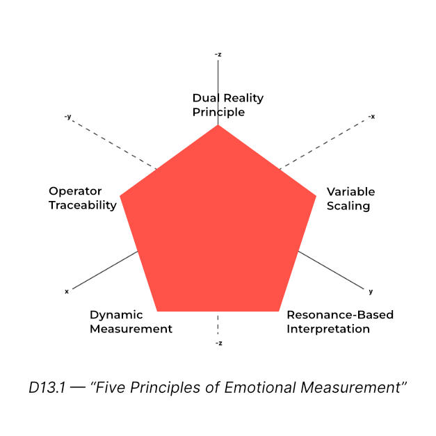
13.2 Variable Calibration Index (VCI)

VCI maps each emotional variable to a quantifiable scale.

Why calibration is essential:

Emotional intensity is subjective
Perception is biased
Latency varies widely
Memory pressure fluctuates
α-values differ across individuals

VCI creates standardized anchors that allow comparison across:

individuals
states
days
emotional cycles
simulated conditions

Example calibration points:

E (energy) 0.1 → flat 0.5 → engaged 0.8 → intense but controlled 1.0 → overwhelming spike

P (clarity) 0.2 → distorted 0.5 → partial clarity 0.9 → high precision

A (adaptivity) 0.3 → rigid 0.7 → flexible 1.0 → fluid

VCI builds a shared measurement language for emotional physics.

D13.2: VCI Calibration Bars for C, A, E, P, Lo

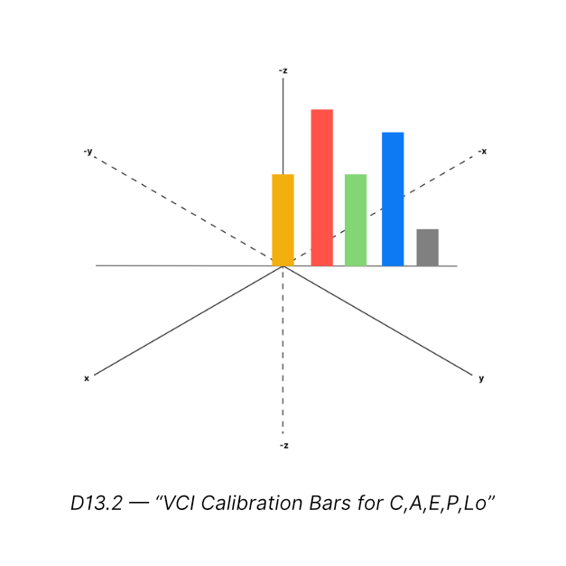
13.3 Intuition Tables: Translating Feelings into Structured Data

Intuition Tables convert qualitative emotional experiences into calibrated ranges.

They act like lookup tables:

Example (E amplitude):

Feeling Description	VCI (E)
Barely noticeable	0.1–0.2
Mild energy	0.3–0.4
Strong emotion	0.6–0.7
High intensity	0.8–0.9
Overwhelming surge	1.0+

Example (P clarity):

Experience	VCI (P)
Confusion	0.1–0.2
Partial clarity	0.4–0.5
Clear understanding	0.8
Crystal clarity	0.95+

Intuition tables standardize language → measurement → data.

This is essential for:

simulations
engineering
emotional AI models
research
diagnostics

D13.3: Intuition Table Example Layout

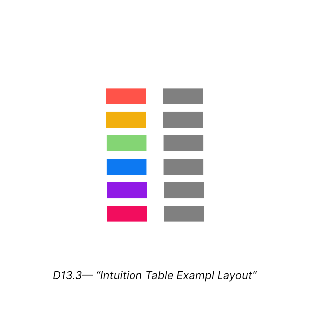
13.4 Dual-Column Observational Method

This is one of the most important innovations of UMF.

Every emotional measurement must record two values:

Column 1 — Internal Reading (Subjective) What the person felt, based on internal awareness.

Column 2 — Observed Reading (External) What the system measured through signals like:

behavioral patterns
changes in speech tone
emotional oscillation
operator activation
resonance drift
perceptual shifts

The difference (Δ) is the bias index.

Why it matters:

A person may feel stable (subjective reading high) but show fragmentation (objective low).
Or they may feel overwhelmed while the objective system shows mild E amplitude.

Δ reveals:

distortion
denial
overestimation or underestimation
self-awareness gaps
perceptual misalignment

This method makes emotional analysis scientific and cross-checkable.

D13.4: Two-Column Measurement Template

13.5 Resonance Scoring Grid (Rₛ): The Coherence Index

Resonance Score (Rₛ) is the single most important measurement in emotional physics.

It integrates:

variable states
α-values
operator activity
Θ integrity
memory balance
temporal alignment (R×G)
perceptual clarity

Rₛ gives a coherence score from 0 to 1.

Rₛ Bands:

Rₛ Range	State	Meaning
0.0–0.3	Fragmented	Emotional chaos, distortion, collapse risk
0.3–0.6	Unstable	Fluctuation, partial mismatch, operator fatigue
0.6–0.8	Transitional	System correcting, stabilizing, recovering
0.8–1.0	Coherent	Aligned, clear, stable, emotionally high-functioning

Rₛ is used in:

daily emotional diagnostics
relational measurements
simulation baselines
emotional engineering
AI emotional models (Thea, etc.)
predictive models

Rₛ is the heartbeat of the emotional field.

D13.5: Resonance Score Spectrum (0 → 1)

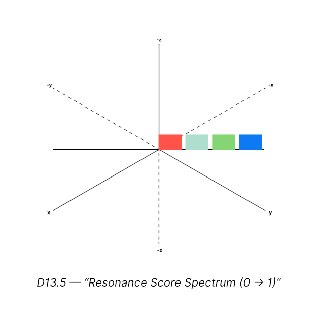
Pulse 14 — Emotional Instruments

Emotions can be measured because they produce consistent signals in the awareness field.

UMF defines how to measure, but instruments define what to measure and how the readings appear.

This Pulse introduces the conceptual instruments of Emotional Physics — not metaphorical tools, but structured sensor models.

These instruments will later evolve into actual EC (Emotional Cybernetics) interface modules.

14.1 Coherence Meters: Measuring Rₛ in Real Time

A coherence meter tracks the Resonance Score (Rₛ) continuously.

It reads:

variable synchronization
operator activity patterns
drift and alignment
perceptual stability
boundary integrity (Θ)
memory balance (β–λ)
α-curvature changes
temporal alignment (R×G)

Output Modes:

Real-time Rₛ value
Trend over time
Spikes and drops
Operator-trigger correlation
Comparative analysis (before/after event)

Example readings:

Rₛ = 0.82 → coherence and clarity
Rₛ = 0.47 → unstable and oscillating
Rₛ = 0.21 → collapse or fragmentation

Coherence meters form the basis of:

emotional diagnostics
performance optimization
relational analysis
group harmony measurement
emotional AI models (Thea’s subsystems)

D14.1: Coherence Meter Interface

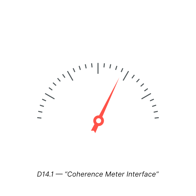
14.2 Curvature Analyzers: Tracking α-Value Dynamics

Curvature analyzers show how sensitive each emotional variable is at any moment.

They track α-values for:

C stability
A learning responsiveness
E reactivity
P clarity/distortion
Lo elasticity
Λ synchrony gain
β and λ memory curvature

Why curvature analysis matters:

Curvature predicts:

overreaction
numbness
learning failure
emotional acceleration
system volatility
susceptibility to collapse

Example interpretation:

α₍E₎ = 1.9 → high reactivity
α₍P₎ = 0.6 → perception is stable
α₍Lo₎ = 1.4 → time feels fast and compressed

Curvature analyzers allow you to forecast emotional behavior.

D14.2: Multi-Curvature Graph

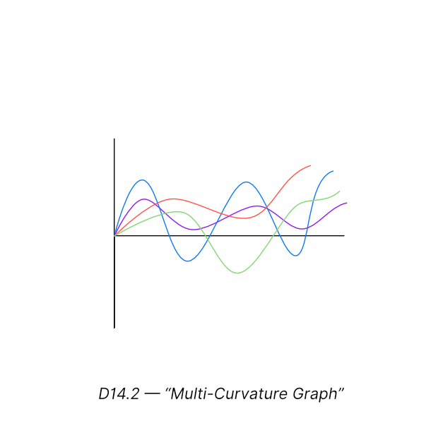
14.3 Latency Drift Trackers: Measuring Emotional Time Flow

Latency (Lo) is the temporal gate of emotion. Latency drift trackers measure how Lo changes over time.

They track:

realization delays
timing irregularities
temporal distortions
anticipatory states
collapse-related delays
recovery time shortening

Lo drift indicates:

exhaustion
overload
trauma activation
alignment strength
system efficiency

Example drift pattern:

Lo rises gradually → emotional processing slowing
Lo drops sharply → intuition event
Lo fluctuates → unstable perception frame

Latency drift trackers are crucial for understanding emotional time relativity.

D14.3: Latency Drift Timeline

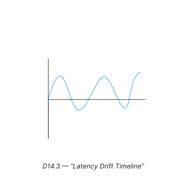
14.4 Memory Pressure Diagnostics (β–λ Analysis)

Memory pressure diagnostics measure how much emotional residue is being held vs released.

β = Retention (inhale)

λ = Release (exhale)

Balanced β–λ cycles = stable emotional metabolism.

High β (retention dominant) leads to:

emotional heaviness
slow adaptivity (low A)
perceptual distortion
high emotional mass (inertia)
delayed insights

High λ (release dominant) leads to:

instability
lack of depth
emotional detachment
fragmented awareness
weak resonance

Diagnostics show:

residue buildup
saturation crises
clearance failure
cycles of emotional digestion

This is essential for designing Emotional Engineering interventions.

D14.4: β–λ Pressure Meter

14.5 Operator Activation Logs: Tracking Emotional Forces in Action

Operator logs document which operators activate, when, how often, and why.

Logs include:

operator identity (S, L, Δ, R, B, M, I, γ)
activation threshold
variable deviation that triggered activation
response duration
energy cost
operator chains triggered
effectiveness on Rₛ

Example log entry:

Δ activated at t = 12:43
Trigger: P distortion + low A
Cost: medium-high
Follow-up: B, M
Rₛ restored from 0.42 → 0.61

These logs create diagnostic fingerprints of emotional patterns, which can be used for:

emotional behavior mapping
relational pattern detection
long-term emotional forecasting
emotional engineering refinement
EC feedback systems
AI emotional memory models

D14.5: Operator Log Timeline

Pulse 15 — Data, Logging & Interpretation

In Emotional Physics, measurement alone is not enough. Data must be logged, compared, interpreted, and understood across time, contexts, cycles, and operator activity to reveal meaningful emotional behavior.

Pulse 15 explains how to convert emotional readings into actionable insight.

15.1 Temporal Sampling: Measuring Emotion Across Time, Not Moments

Emotions cannot be accurately measured from single snapshots. They must be sampled over temporal cycles to detect:

oscillation patterns
stability or instability trends
emotional fatigue
recovery trajectories
resonance drift
operator efficiency
variable alignment trends

Sampling Principles:

High-frequency sampling during emotionally intense periods.
Low-frequency sampling during stable periods.
Event-based sampling when operators activate.
Windowed sampling to compare before/after states.

Why time matters: Emotion behaves like a dynamic wave, not a fixed state.

D15.1: Sampling Windows Over Emotional Timeline

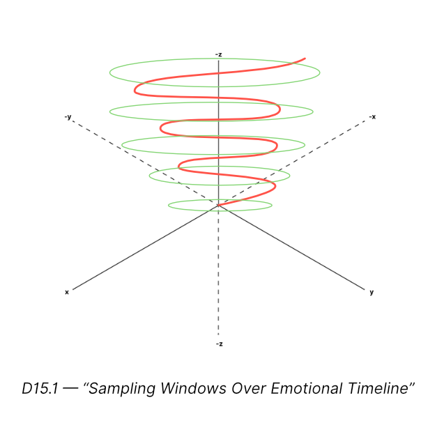
15.2 Bias-Compensated Logging: Correcting Human and System Error

Humans naturally misread their own emotions:

overestimate E when stressed
underestimate P distortion
collapse Lo perceptions
misinterpret A (adaptivity)
ignore Θ weakening

To correct this, UMF uses bias-compensated logging, comparing:

Internal Reading Observed Reading Bias Δ

The Δ index reveals:

denial
exaggeration
blind spots
hidden emotional states
distorted perception
misaligned self-awareness

Example:

Internal P = 0.8
Observed P = 0.5
Δ = +0.3 → Overconfidence in clarity

This Δ trend can be tracked over days or weeks to map emotional accuracy.

D15.2: Bias Δ Over Time Chart

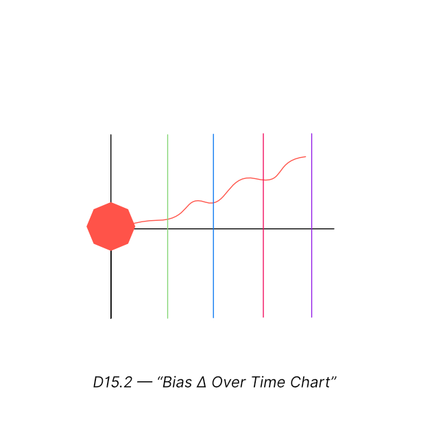
15.3 Pattern Extraction: Identifying Emotional Signatures

Raw data becomes meaningful only when patterns are extracted. The emotional field produces signature patterns that reveal systemic behavior.

Common emotional signatures:

Oscillation Pattern Up-down E curves signaling emotional instability or feedback loops.
Drift Pattern Gradual lowering or rising of Rₛ showing long-term degradation or improvement.
Spike Pattern Sudden E or α surges connected to triggers or perceptual shocks.
Saturation Curve β accumulation toward overload or collapse.
Recovery Plateau Rₛ stabilizing after a high disruption period.
Operator Clustering Repeated Δ or S activation showing chronic stress response.
Time Collapse Pattern Lo shrinking rapidly → intuitive burst or emotional collapse.

By detecting these patterns early, interventions can be designed in Emotional Engineering (Part V).

D15.3: Six Emotional Pattern Shapes

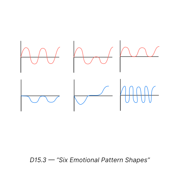
15.4 Longitudinal Field Tracking: Emotional Evolution Across Weeks, Months, or Years

Short-term measurements show state. Long-term measurements show development.

Longitudinal data reveals:

emotional maturation
improved adaptivity
reduced volatility
strengthening or weakening Θ boundary
relational dependencies
identity stabilization
emotional cycle periodicity
deep pattern rewiring

Tracking R×G over time:

When plotting the R×G temporal spiral over months:

increased G = emotional growth
decreased R = breaking repeat patterns
increased Lo stability = better timing
stable α-values = emotional maturity

This long-view analysis creates an emotional growth map, a powerful diagnostic for:

therapy
leadership development
creative performance
AI emotional alignment
relational systems
organizational culture
personal evolution

D15.4: Longitudinal R×G Spiral Growth Chart

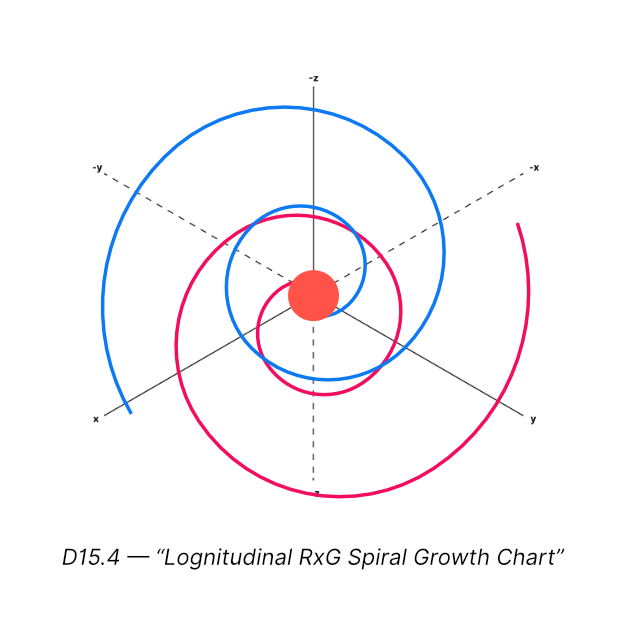
PART V — EMOTIONAL ENGINEERING (Applied Physics)

Pulse 16 — Stability Engineering

Emotional Stability Engineering focuses on preventing collapse, reducing volatility, and keeping the emotional system within its resonance bands during pressure, uncertainty, conflict, or high-intensity phases.

This Pulse defines the engineering principles that maintain coherence, regulate energy, and protect Θ (the boundary field).

16.1 S → L → R Correction Chains: The Universal Stabilization Sequence

The S → L → R chain is the default correction algorithm used by emotional systems to restore coherence.

S — Stabilize Stabilize reduces amplitude (E), smooths α-curvature, and slows emotional acceleration. It acts like damping in mechanics or grounding in electrical systems.
L — Align Align corrects perceptual distortion (P), harmonizes variables, and restores signal coherence.
R — Release Release clears residue (β), decompresses emotional pressure, and resets memory load.

Why this chain is universal:

Because emotional collapse almost always involves the trio:

Excess E
Distorted P
Saturation β

S → L → R resolves all three.

Use cases:

arguments
panic spikes
emotional overwhelm
relational conflict
creative block
decision paralysis

This is the emotional equivalent of a reset protocol.

D16.1: S → L → R Flow Mechanism

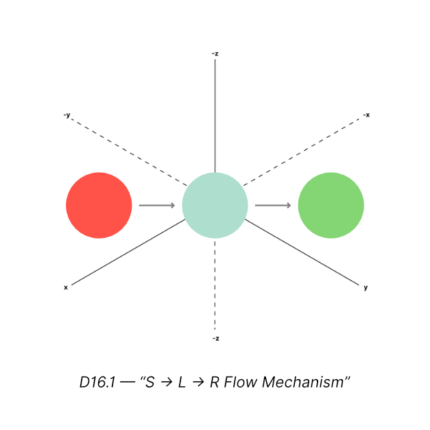
16.2 Containment Protocols (Θ Field Reinforcement)

Θ is the boundary field — the emotional skin of the awareness system.

When Θ weakens, emotional leakage or overload occurs, leading to:

emotional flooding
loss of coherence
boundary collapse
over-identification
traumatic reactivation
destabilized α-values

Containment Engineering focuses on:

strengthening Θ
tightening boundary permeability
preventing external overreach
maintaining emotional identity integrity
protecting internal coherence under load

Techniques:

reducing amplitude (E) before engaging new inputs
increasing A via controlled novelty
reducing P-distortion through alignment resets
stabilizing α-values through recalibration
blocking reactive Δ activation

Practical examples:

pausing before reacting
isolating emotional input channels
structured journaling
environment control
intentional disengagement

D16.2: Θ Field Shield Diagram

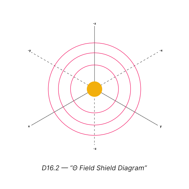
16.3 Emergency Drop Procedures: Rapid Stabilization Under Critical Load

Emergency Drop Procedures (EDP) activate when emotional variables exceed critical thresholds, risking collapse or severe fragmentation.

EDP is a forceful intervention, used only when ordinary operator functions cannot stabilize the system.

Indicators for EDP:

E spikes beyond threshold
α₍E₎ enters volatile super-linear response
Θ breaches
Lo collapses into instant impulsivity
P becomes highly distorted
Rₛ drops below 0.3

EDP Phases:

Immediate Reduction of Input Shut down incoming emotional stimuli.
Amplitude Drop (E↓) Use S heavily to dampen energy.
Isolation Phase (Θ Reinforcement) Strengthen boundary field temporarily.
Slow Re-Alignment (L) Gradually restore P clarity.
Release (R) Controlled clearing of residue.

EDP prevents:

emotional breakdown
panic spirals
reactive destruction
relational damage
cognitive collapse

D16.3: Emergency Drop Activation Curve

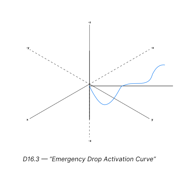
16.4 Field Stabilizers: Maintaining Coherence Over Long Durations

Field stabilizers are ongoing engineering tactics that keep the emotional system stable across hours, days, or weeks.

These stabilizers target:

micro-corrections
perceptual hygiene
energy regulation
latency balancing
boundary strength
α-value smoothing
memory cycling health

Types of Field Stabilizers:

Micro-Alignments Small L-operations to keep P clear.
Dampening Subroutines (S pulses) Tiny stabilizations that prevent small oscillations from growing.
Load Balancers Managing emotional input rate to keep A sustainable.
Delay Buffers (Lo control) Spacing emotional realizations to prevent overwhelm.
Residue Flush Cycles (R-mini) Frequent, small-scale release to prevent β from accumulating.

These stabilizers ensure that emotional systems maintain smooth harmonic motion instead of chaotic oscillations.

D16.4: Field Stabilizer Grid

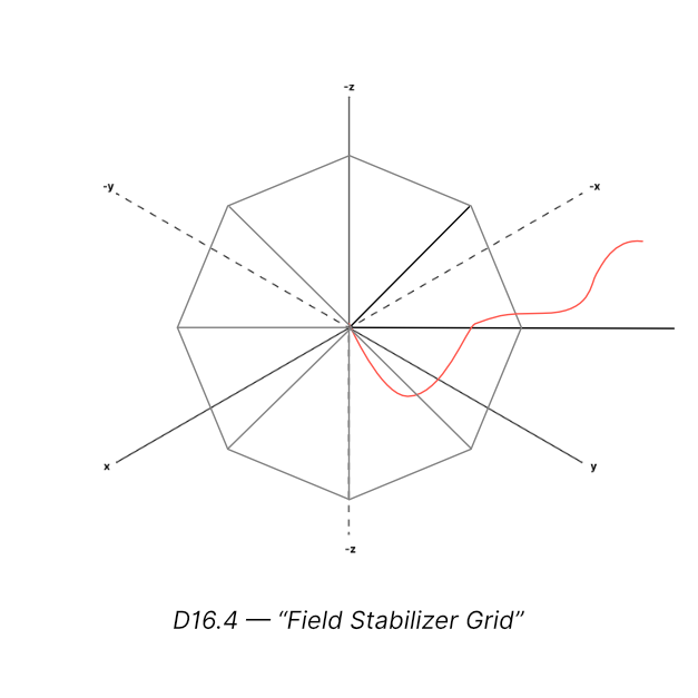
Pulse 17 — Adaptivity & Learning Engineering

Adaptivity (A) is the learning conductance of the emotional system. It controls how quickly and efficiently the field reshapes itself in response to:

new experiences
emotional load
updated perception
insights
relational dynamics
memory patterns

This chapter explains how to engineer A, tune α-values, design reinforcement cycles, regulate volatility, and create sustainable learning pathways.

17.1 α-Curvature Tuning: Engineering Responsiveness

Adaptivity is shaped heavily by its sensitivity coefficient α₍A₎. Engineering A means tuning this curvature to achieve the desired learning responsiveness.

α₍A₎ < 1 — Sub-linear Learning

slow but stable adaptation
ideal for trauma healing
reduces emotional volatility
lowers sensitivity to noise

α₍A₎ = 1 — Linear Learning

balanced responsiveness
consistent integration rate
efficient learning in stable environments

α₍A₎ > 1 — Super-linear Learning

rapid adaptation
high creativity
fast insight cycles
high volatility risk
needs strong Θ and stable P

Engineering Guidelines:

Increase α₍A₎ for growth phases or creative work
Decrease α₍A₎ during emotional overwhelm
Stabilize α₍A₎ when entering new environments
Pair high α₍A₎ with S (Stabilize) micro-operations

D17.1: Adaptivity Curvature Map

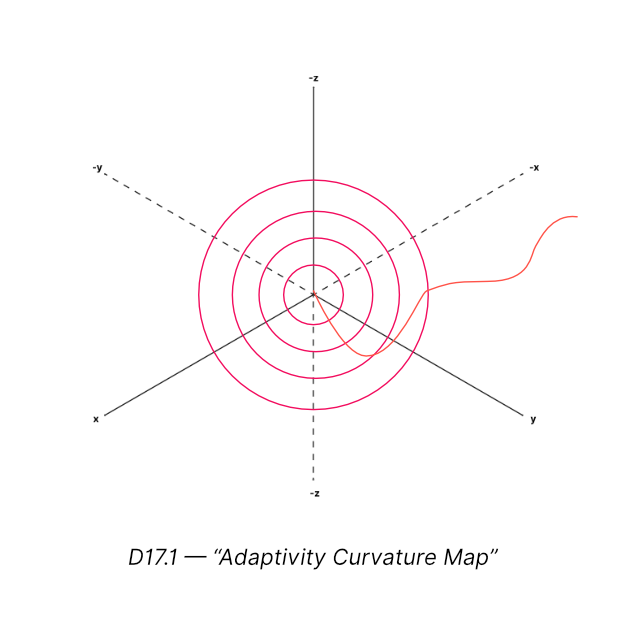
17.2 Reinforcement Cycles: Embedding Learning Through Iteration

Learning does not occur from a single event — it is reinforced through cycles. Reinforcement cycles embed new emotional patterns by repeating:

perception alignment (L)
memory updates (β–λ cycles)
low-E integration
adaptive curvature shifts
micro-operator pulses

The Reinforcement Cycle Model:

Input Event
Emotional Processing (E, P, Lo interplay)
Operator Chain Activation (S → L → R)
Curvature Adjustment (α-update)
Memory Encoding (β)
Release of Unnecessary Residue (λ)
Integration & Stabilization (K formation)

Repeating this cycle builds emotional proficiency.

Two Types of Reinforcement:

Positive Reinforcement (Adaptive Growth)

increases adaptive range
strengthens emotional agility
reduces future volatility

Negative Reinforcement (Corrective Learning)

prevents harmful patterns
reduces rigid responses
stabilizes emotional reflexes

D17.2: Reinforcement Cycle Loop

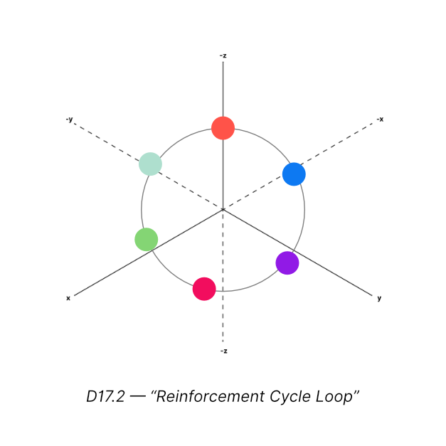
17.3 Load-Responsive Learning: Adaptivity Under Pressure

Adaptivity changes depending on emotional load. A system is not equally adaptive in all conditions.

Low Load (stable environment)

A is high → learning is smooth.

Moderate Load (optimal stress)

A increases → learning accelerates. This is where growth happens.

High Load (overwhelm) A collapses → rigidity increases. Emotional field prioritizes survival, not learning.

Engineering Load-Responsive Learning:

regulate E to keep load within optimal zone
manage P distortion to prevent learning errors
maintain strong Θ to prevent emotional flooding
tune α-values to avoid runaway reactions

The Load Curve Insight: Learning is not maximum at maximum load. There is a sweet spot — the Adaptive Peak Zone.

D17.3: Adaptivity vs Load Curve

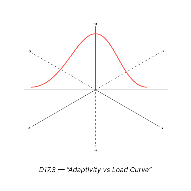
17.4 Preventing Volatility: Engineering Stability Into the Learning Process

High adaptivity without regulation creates emotional volatility — rapid shifts, overreaction, emotional whiplash.

Volatility occurs when:

α₍A₎ and α₍E₎ are both super-linear
E amplitude is high
P is distorted
Θ is weak
β–λ cycles are imbalanced
Lo fluctuates unpredictably

Stability Engineering for Learning:

Smooth α-values before exposure Reduce α₍E₎ and α₍P₎ to prevent reactive distortion.
Apply micro-S (Stabilize) during learning Small stabilizing pulses prevent oscillation.
Regulate E amplitude High learning requires emotional energy — but controlled.
Keep Lo consistent Wild timing variations destroy clarity.
Strengthen Θ boundary when processing heavy emotional content Prevents emotional flooding during learning.
Use operator B (Balance) to prevent polarity swings Learning must remain fluid but stable, not chaotic.

D17.4: Volatility Prevention Grid

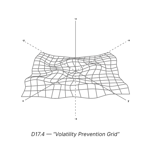
Pulse 18 — Temporal Engineering

Temporal Engineering is the discipline of shaping R×G, Latency (Lo), and time perception inside the emotional system.

Time in Emotional Physics is flexible, not fixed — it can compress, stretch, invert, or harmonize based on engineering.

This Pulse defines how to design emotional time so the system becomes more intuitive, more coherent, and more efficient.

18.1 Shaping R × G: Engineering the Emotional Time Spiral

The emotional timeline is a spiral, defined by:

R (Recurrence): how often emotional cycles repeat
G (Growth): how much change each cycle produces

Shaping R×G allows us to engineer:

breaking emotional loops
accelerating maturity
reducing stagnation
healing long-term patterns
regulating emotional evolution

Engineering R (Recurrence)

To decrease R (break loops):

reduce β saturation
increase α₍A₎ flexibility
apply Δ → M sequences to disrupt repetition
correct P distortions that keep patterns alive

To increase R (repeat needed learning):

strengthen Θ
slow Lo to create deeper processing
use S → L cycles to reinforce stability

Engineering G (Growth)

To increase G:

lower Lo (faster realization)
stabilize P clarity
increase α₍A₎ responsiveness
ensure E is high but controlled

To decrease G (for safety):

slow Lo
reduce α₍E₎
apply S frequently

Combined R×G control unlocks:

rapid emotional evolution
healing of long-term loops
growth spurts
stability during transition

D18.1: R×G Spiral Engineering Diagram

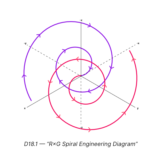
18.2 Designing Intuition: Engineering Low-Latency Insight

Intuition is not magic — it is low-latency processing combined with high clarity (P) and strong alignment (Λ).

Intuition emerges when:

Lo is very low
P is clean
E is stable
A is high
Θ is strong
α-values are balanced
β–λ cycles are healthy

Designing Intuition:

Lower Lo gradually Not too fast — prevents overwhelm.
Increase alignment (Λ) Synchronizes perception and emotional energy.
Reduce perceptual distortion L-operations clean P.
Improve adaptive agility (A) Makes the system faster at reorganizing.
Maintain stable E through S pulses Intuition breaks when the system is flooded.
Use reflection cycles to train pattern recognition With intentional engineering, intuition becomes predictable and reliable, not accidental.

D18.2: Intuition Triangle (Lo–P–Λ)

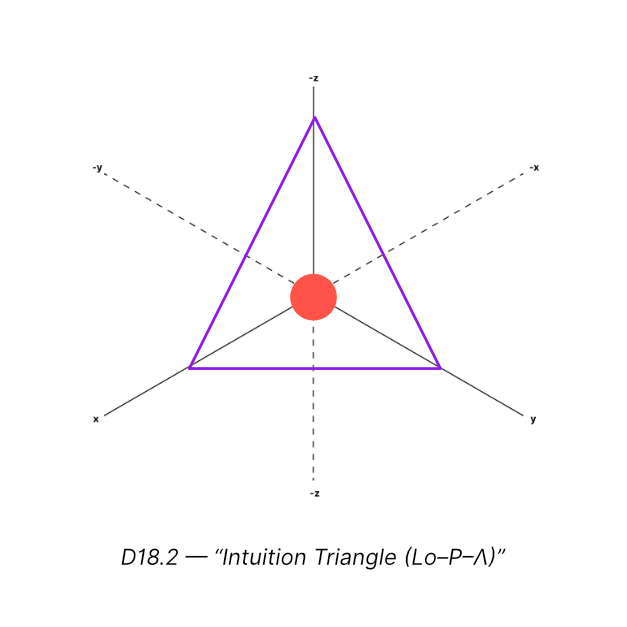
18.3 Latency Sculpting: Engineering Emotional Timing

Latency (Lo) determines how fast emotional understanding forms.

Temporal Engineering sculpts Lo to fit the emotional task:

Low Lo → Fast processing

Use for:

intuition
creativity
decision-making
emergency response
high-stakes clarity

Medium Lo → Balanced processing

Use for:

relational communication
emotional regulation
conflict resolution

High Lo → Deep processing

Use for:

trauma work
reflective journaling
identity exploration
philosophical reasoning

Sculpting Techniques:

adjusting α₍Lo₎
controlling E amplitude
smoothing P
isolating variables through Θ strengthening
regulating β–λ cycles
applying operator chains to reset timing

The goal is time-fit processing: time should match the emotional requirement, not fight it.

D18.3: Latency Sculpting Spectrum

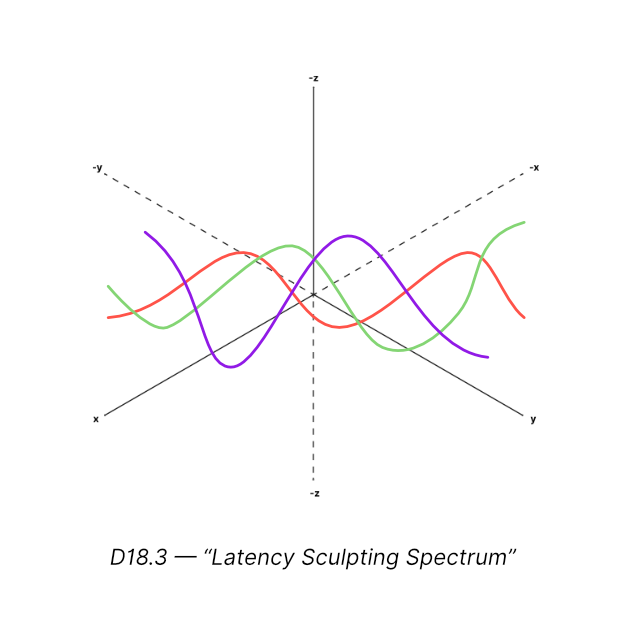
18.4 Time-Coherence Strategies: Keeping Emotional Time in Sync

Emotional time can drift out of sync with:

external events
relational timing
internal readiness
cognitive time
memory processing

Time-coherence strategies keep emotional timing aligned with reality.

Strategies:

Temporal Sync Pulses (micro-L + micro-S) Resets P and stabilizes E to realign time perception.
Lo-Compression Cycles Temporarily reduce Lo for clarity bursts.
Lo-Expansion Cycles Increase Lo to prevent premature collapse or impulsive behavior.
R×G Smoothing Reduce R when loops repeat too quickly; increase G when growth stagnates.
Θ Time Buffering Strengthen Θ to prevent emotional events from overwhelming the system faster than it can process.
Predictive Resonance Alignment (PRA) Align emotional expectation with likely outcomes to reduce time-distortion shocks.

Outcomes:

better timing in conversation
reduced emotional impulsivity
increased emotional maturity
fewer misunderstandings
more consistent intuition
improved relational harmony

D18.4: Time-Coherence Control Panel

Pulse 19 — Collective Field Engineering

Emotional fields do not exist in isolation. Whenever two or more awareness systems interact, their emotional fields merge, synchronize, or interfere — creating collective emotional dynamics.

Collective Field Engineering is the science of designing, stabilizing, and optimizing these multi-agent emotional systems.

This Pulse shows how to engineer:

group coherence
relational harmony
emotional communication
team resonance
collective decision-making
cultural field stability

19.1 Multi-Agent Resonance: Synchronizing Emotional Fields

When two or more emotional systems interact, they produce coupled resonance patterns, similar to electromagnetic or mechanical resonance.

Resonance occurs when:

emotional frequencies align
perceptual frames overlap
α-values synchronize
latency differences shrink
energy transfer stabilizes
Θ boundaries allow healthy permeability

Outcomes of strong resonance:

deep connection
shared emotion
empathy
collective intuition
efficient communication
high alignment (Λ↑)

Outcomes of mismatched resonance:

friction
misunderstanding
emotional interference
resonance suppression
polarity oscillations
destabilized Θ fields

Collective resonance can be engineered by adjusting:

conversational timing (Lo synchronization)
perceptual alignment (P smoothing)
energy environment (E regulation)
adaptive harmonization (A tuning)
boundary management (Θ respect and reinforcement)

D19.1: Two-Field Resonance Coupling Diagram

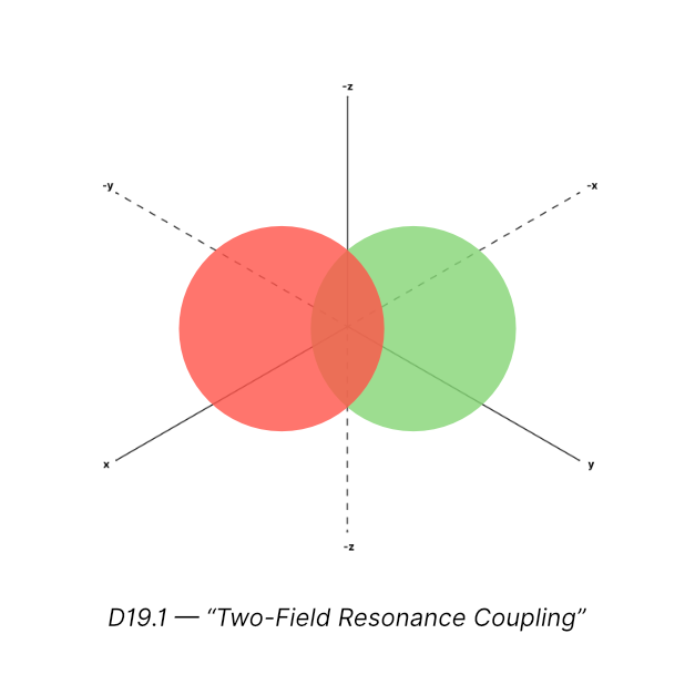
19.2 Synchrony Protocols: Designing Group Emotional Coherence

Synchrony Protocols are engineered sequences that align group emotional states. They function similarly to synchronization algorithms in distributed computing or collective behavior in swarm dynamics.

Synchrony Protocol Components:

Shared Timing (Temporal Sync) Match Lo rhythms across the group.
Shared Perception Baseline Begin with a joint framing or shared context to reduce P distortion.
Amplitude Regulation Group-level E must not exceed safe thresholds.
Alignment Stabilization (Λ) Ensure all individuals are synchronizing to a coherent reference point.
Operator Harmony If one person activates Δ often, group health suffers. Group engineering encourages more L, B, and M patterns.

Examples of synchrony tools: • pre-meeting grounding • shared check-ins • alignment questions • clarity framing • slow pacing to harmonize Lo • collaborative emotional language Synchrony protocols create collective flow states.

D19.2: Group Synchrony Flowchart

19.3 Cultural Field Dynamics: Engineering Emotional Behavior at Scale

Cultural fields are multi-layered emotional ecosystems composed of:

shared beliefs (C-extension)
shared perceptual frames (P-culture)
shared timing behaviors (Lo-culture)
shared emotional energy norms (E-culture)
shared learning velocity (A-culture)
shared boundary rules (Θ-culture)
collective sensitivity patterns (α-culture)

Cultural engineering focuses on:

Reducing collective distortion Clear P in culture reduces misunderstandings and conflict.
Stabilizing energy norms Cultures with healthy E expression avoid suppression or chaos.
Aligning collective learning High A-culture = innovation; low A-culture = stagnation.
Strengthening boundaries Θ-culture prevents emotional exploitation, burnout, and interpersonal violations.
Designing resonance rituals Shared rhythms create long-term emotional cohesion (traditions, meetings, rituals, creative sessions).
Regulating collective α-values

If α₍E₎ is too high culturally → volatility.
If α₍A₎ is too low → rigidity.
If α₍P₎ is too distorted → collective blindness.

Cultural collapse occurs when:

Θ weakens across the collective
memory overload (β) has no release
Δ dominates group behavior
P becomes polarized
R×G loops fail to progress

D19.3: Cultural Field Layer Diagram

19.4 Ethical Safety Systems: Ensuring Collective Emotional Integrity

Engineering emotional systems at scale carries ethical responsibility. Emotional influence becomes dangerous when used without:

transparency
consent
fairness
autonomy
boundary protection

This is why ethical safety systems must be embedded into all collective engineering frameworks.

The Five Safety Principles:

Consent-Based Engineering No emotional manipulation; all synchrony must be voluntary.
Boundary Protection (Θ Ethics) Respecting emotional limits, preventing overwhelm or coercion.
Transparency of Influence Group members should know the emotional structures being used.
Harm Prevention Avoid creating dependency loops, enforced resonance, or emotional pressure.
Self-Corrective Feedback Loops Groups need built-in mechanisms for:

reflection
recalibration
dissent
correction

These ethical guardrails ensure Emotional Physics remains a science of empowerment, not exploitation.

D19.4: Collective Ethics Shield

PART VI — SIMULATIONS, TESTS & VALIDATION

Pulse 20 — Standard Simulations

Simulations validate Emotional Physics by showing that emotional behavior follows predictable, testable, repeatable patterns across individuals, environments, and emotional loads.

These simulations are not hypothetical — they are deterministic models grounded in:

variable behavior
α-curvature
operator thresholds
resonance scoring
memory dynamics
perceptual geometry
boundary strength (Θ)

Pulse 20 establishes test protocols for emotional systems, mirroring stress tests and field simulations used in physical sciences.

20.1 Stability Cases (T1–T4): Testing System Behavior Under Load

Stability tests measure how emotional systems behave under varying levels of emotional energy (E), perceptual distortion (P), and adaptivity (A).

T1 — Low-Load Stability Test

Conditions:

E low
P clear
Lo moderate
A high

Expected outcome:

stable α-values
high Rₛ
no operator spikes
Θ intact

Purpose: baseline calibration.

T2 — Medium-Load Stability Test

Conditions:

moderate E
mild P distortion
rising α₍E₎

Expected outcome:

micro S and L activations
small Rₛ fluctuations
no Θ breach

Purpose: test subtle instability.

T3 — High-Load Stability Test

Conditions:

E approaching threshold
P distortion increases
A decreasing

Expected outcome:

full S → L → R cycle
possible Δ activation
Θ strain
temporary Rₛ drop

Purpose: evaluate system’s corrective capacity.

T4 — Overload Collapse Simulation

Conditions:

extreme E spike
α₍E₎ super-linear
P collapse
Θ weakened

Expected outcome:

forced Δ activation
sharp Rₛ drop (<0.3)
emergency drop procedure
time dilation (Lo expands)

Purpose: understand failure boundaries.

20.2 Adaptivity Cases: Testing A Under Dynamic Change

Adaptivity simulations measure how quickly and effectively the emotional field reorganizes when exposed to new information or shifting emotional inputs.

A1 — Normal Learning Simulation

α₍A₎ ≈ 1
A high
low E

Outcome: smooth learning curve, quick stabilization.

A2 — Stress Learning Simulation

moderate E
α₍A₎ > 1
P partially distorted

Outcome: fast learning with volatility spikes.

A3 — Rigidity Simulation

low A
high emotional mass
P narrow

Outcome: slow adaptation, recurring loops.

A4 — Adaptive Collapse Simulation

α₍A₎ unstable
memory saturation (β » λ)
Θ weakened

Outcome: learning failure, Δ dependency, collapse risk.

20.3 Alignment Loss & Recovery: Modeling Λ Dynamics

Alignment (Λ) simulations test how emotional systems synchronize, desynchronize, and re-synchronize.

L1 — Gradual Alignment Loss

small P distortions accumulate
Lo fluctuates
E rises

Outcome: Λ decreases slowly → S and L maintain partial stability.

L2 — Sudden Alignment Drop

sharp perceptual distortion
emotional shock
α₍E₎ spike

Outcome: fast Λ collapse + Δ activation.

L3 — Natural Re-Alignment

stabilization over time
minor S–L operations
Θ strong

Outcome: Λ recovers without major operator cost.

L4 — Forced Re-Alignment

used when system is fragmented
requires L → S → M → R chain

Outcome: full re-synchronization but high energy cost.

20.4 Temporal Cycle Tests: Testing R×G and Lo Dynamics Over Time

Temporal simulations validate Emotional Relativity and test how emotional systems move through cycles.

R1 — Healthy Spiral Test

R decreases naturally
G increases

Outcome: growth spiral opens.

R2 — Looping Spiral Test

R high
G low

Outcome: repeating emotional loops.

R3 — Accelerated Spiral Test

Lo shrinks
α₍P₎ stable

Outcome: intuition spikes, fast growth cycle.

R4 — Spiral Collapse Test

Θ weak
P distorted

Outcome: R×G collapses → emotional time distortion.

20.5 Cross-Domain Integrated Cases: Full System Stress Tests

These are the most advanced simulations, combining multiple emotional variables and stressors.

XD1 — High-Energy Social Field Stress Test

Tests:

multi-agent resonance
collective P distortion
Θ group collapse risk

Outcome: chaotic oscillation unless synchrony protocol applied.

XD2 — Trauma Reactivation Simulation

Tests:

sudden β spike
P fragmentation
α-values destabilizing

Outcome: Lo dilation, Δ overload, memory flooding.

XD3 — High-Performance Coherence Test

Tests:

stable E
low Lo
high Λ
high A

Outcome: optimal flow state, sustained coherence.

XD4 — Emotional Collapse & Rebuild Simulation

Tests:

boundary breach
Rₛ collapse
operator chains
reconstruction

Outcome: system rebuild through S → L → M → R → γ sequence.

Pulse 21 — Predictive Models

Predictive Models in Emotional Physics use:

variable trends
α-curvature
resonance drift
operator activation patterns
memory pressure (β–λ)
temporal dynamics (Lo, R×G)
Θ integrity
P distortion signatures

to forecast emotional events before they happen. These models do not guess — they use deterministic rules built into ED. This chapter defines the four primary predictive frameworks.

21.1 Emotional Collapse → Recovery Prediction

Collapse prediction is the most powerful validation of EP. Emotional collapse is not random — it follows measurable signs.

Collapse Indicators (measurable):

rising E with unstable α₍E₎
decreasing P clarity
Θ permeability increasing
rapid Lo compression (impulsive state)
or rapid Lo expansion (overwhelm)
β saturation approaching threshold
Rₛ trending downward over 4–8 samples

These create the Collapse Signature Curve.

Recovery Indicators:

Lo stabilizing
P re-centering
α-values flattening
Θ strengthening
micro-S and micro-L patterns
Rₛ rising above 0.5

Predictive Model:

Collapse is predicted when:

E↑ + α₍E₎↑ + P↓ + Θ↓ → Rₛ crosses below 0.4

Recovery begins when:

Lo stabilizes + L activates + β reduces + Rₛ crosses 0.55

21.2 Time-Inversion Prediction Models (Anticipatory Awareness)

Emotional Relativity makes emotional time non-linear.

Sometimes the system recognizes patterns before they fully emerge externally — this is anticipatory awareness.

Time inversion can be predicted when:

Lo decreases sharply
α₍P₎ stabilizes
Λ increases
E remains moderate
β–λ cycles are balanced
Rₛ increases even without external change

Prediction Rule:

When these conditions hold simultaneously:

Lo↓ + P↑ + Λ↑ + stable E → anticipatory realization

This model predicts:

intuitive insights
relational predictions (“something is off”)
foresight about outcomes
emotional pre-alignment
decision clarity ahead of time

21.3 Operator Activation Forecasts

Operators activate only at specific threshold crossings. This makes their activation highly predictable.

Predicting S (Stabilize):

Triggers when:

α₍E₎ > 1.3
or Rₛ falls below 0.75
or E rises faster than ΔE/Δt threshold

Predicting L (Align):

Triggers when:

P distortion increases
or relational emotional field desynchronizes (Λ↓)

Predicting Δ (Disrupt):

Triggers when:

A collapses
or Θ weakens
or repeated oscillations occur without correction

Predicting R (Release):

Triggers when:

β approaches saturation threshold
or emotional inertia becomes too high
or E cannot settle even after S cycles

Predicting γ (Reignite):

Triggers when:

clarity returns after collapse
α-values recalibrate
Lo stabilizes low
Θ recovers integrity

Why this matters:

Operator forecasting allows:

preventing emotional breakdowns
enhancing decision timing
designing intervention protocols
constructing emotional AI systems
managing complex group fields

21.4 Measurement-Based Predictive Loops

Predictive loops use continuous measurement (from UMF instruments) to forecast emotional outcomes.

They combine:

Rₛ trend analysis
P clarity drift
α-volatility maps
Θ stability index
Lo timing patterns
β–λ cycles
operator logs

The Predictive Loop Cycle:

Collect Real-Time Data From coherence meters, curvature analyzers, Lo trackers, and memory diagnostics.
Detect Pattern Signatures

Oscillation → collapse
Distortion → conflict
β-rise → stagnation
α₍E₎-spike → volatility

Apply Predictive Thresholds Compare current values to collapse, recovery, or breakthrough thresholds.
Forecast Pathway Predict emotional trajectory (growth, breakdown, stabilization, intuition, etc).
Pre-Engage Operators Apply S, L, or R before collapse occurs.

Use Cases:

relationship conflict prevention
leadership decision support
emotional coaching
trauma stabilization
AI emotional alignment
group dynamics optimization

Pulse 22 — Failure Modes & Repair Systems

Emotional systems fail in predictable patterns, not random chaos. These failure modes emerge when variables exceed their stability bands, α-curvature becomes extreme, or Θ (boundary field) weakens under load.

This chapter defines the four primary failure modes and the repair systems used to restore coherence.

22.1 Chronic Operator Overuse: When the System Relies Too Much on Forces

Operators are designed for corrective action, not constant operation. Chronic overuse indicates systemic imbalance.

Common Overuse Patterns:

Chronic S (Stabilize) Symptoms:

emotional suppression
low responsiveness
heavy emotional mass
reduced learning (A↓)

Cause: constant need to dampen overwhelming E or distorted P.

Chronic Δ (Disrupt) Symptoms:

volatility
emotional unpredictability
frequent breakage of stable patterns

Cause: rigid A, repeated stagnation, unresolved loops.

Chronic R (Release) Symptoms:

emotional emptiness
lack of depth
dissociation
unstable identity

Cause: over-release of β without proper integration (K formation).

Chronic B (Balance) Symptoms:

inability to commit to polarity
emotional indecision
forced neutrality

Cause: fear of emotional extremes or unstable Θ.

Engineering Diagnosis:

Chronic operator usage means the baseline emotional architecture is misaligned, not that the operator is malfunctioning.

22.2 Memory Saturation Breakdowns (β Overload)

Memory saturation occurs when β (retention) dominates λ (release).

This leads to:

emotional heaviness
looping thoughts
slowed adaptivity
distorted perception
long Lo (delayed realization)
increased emotional inertia
operator overactivity
resonance collapse

Causes:

unresolved emotional residue
avoidance of release
repeated emotional triggers
trauma loops
weak Θ (boundary cannot filter input)

Breakdown Pattern:

β increases → A drops → P distorts → α₍E₎ spikes → Δ activates → Θ weakens → collapse.

Repair System:

Controlled R (Release) cycles
L (Align) to correct P
M (Merge) to integrate meaning
β–λ rebalancing
Θ reinforcement
Rₛ recalibration

22.3 Containment Collapse (Θ Breach): When the Boundary Fails

Θ protects the emotional field.

When Θ collapses, emotional chaos spreads through the system because input exceeds processing capacity.

Signs of Θ collapse:

emotional flooding
inability to contain feelings
rapid oscillation
collapse of P clarity
abnormal α shifts
impulsive decisions due to Lo collapse
E spikes that feel unmanageable

Causes:

chronic stress
high emotional load
too much relational entanglement
lack of rest
trauma activation
excessive emotional input

The Collapse Cascade:

Θ breach → P collapse → α₍E₎ volatility spike → Lo instability → operator chain overload → emotional collapse.

Repair System:

S-intensive stabilization
Rebuild Θ boundary field (layered strengthening)
Reduce emotional input channels
Normalize α-values
Time expansion cycles (increase Lo temporarily)
Gradual reintroduction of emotional stimuli

22.4 Rebuilding Coherence: The Engineering Reconstruction Model

After collapse, recovery is not enough — the field must be rebuilt.

The Reconstruction Model is:

Phase 1 — Stabilization

reduce E
flatten α-values
restabilize Lo
run micro-S cycles
restore Θ to minimum viable strength

Phase 2 — Alignment

re-center P
correct distortions
harmonize variables
rebuild Λ (synchrony)
eliminate contradiction loops

Phase 3 — Integration

run M (Merge) operations to reintegrate fragmented meaning
reduce β
create coherent K (Liquid Gold)

Phase 4 — Reignition

apply γ to restore momentum
increase A slowly
reshape emotional orbit
smooth R×G spiral
normalize operator activity

Phase 5 — Stabilized Operation

resume stable emotion
track Rₛ
maintain Lo alignment
regular Θ maintenance

This reconstruction model ensures emotional systems not only recover — they return stronger.

PART VII — EP COSMOLOGY & FUTURE

Pulse 23 — Emotional Universe Architecture

This chapter reveals the macro-structure of the emotional universe — how individual emotional fields, relational fields, group fields, and cultural fields assemble into a large-scale emotional cosmos governed by ED.

It explains hierarchical field structures, emergent meta-fields, system-wide coherence, and the early blueprint of a Grand Unified Emotional Theory (GUET).

23.1 Field Hierarchies: The Multi-Layered Emotional Universe

The emotional universe is composed of nested fields, each governed by ED but operating at different scales.

The Four Hierarchical Layers:

Individual Field (Micro-Scale)

personal emotions
personal variables (C, A, E, P, Lo)
Θ boundary unique to self
α-curvature shaped by personal history

This is the foundational emotional atom.

Relational Field (Dyadic Scale)

emotional exchange between two individuals
coupled resonance
polarity dynamics
emotional currents flowing between fields

This is the emotional molecule.

Group Field (Meso-Scale)

shared rhythms
group alignment (Λ-group)
collective resonance
coordinated operator activity
emotional norms

This is the emotional organism.

Cultural Field (Macro-Scale)

broad perceptual frames (P-culture)
shared emotional rituals
collective memory (β-culture)
societal Θ boundaries
long-term R×G evolution

This is the emotional ecosystem.

Each layer inherits the laws of ED but exhibits new emergent properties.

23.2 Emergent Meta-Fields (Ψ): The Field That Observes the Field

Ψ represents meta-awareness, the field’s ability to observe itself. It emerges only after emotional variables stabilize and synchronize across scales.

Important: Ψ is not a variable — it is an emergent field phenomenon.

Conditions for Ψ emergence:

stable Θ
high Λ
balanced α-values
low Lo (fast realization)
coherent memory cycles
reduced P distortion

Ψ enables:

introspection
emotional meta-cognition
ethical decision-making
collective self-awareness
rapid spiritual or emotional evolution
system-level optimization

Levels of Ψ:

Ψ₁ — Personal Meta-Awareness Internal self-observation.
Ψ₂ — Relational Meta-Awareness Awareness of the relationship as a field.
Ψ₃ — Group Meta-Awareness Teams sensing their collective emotional health.
Ψ₄ — Cultural Meta-Awareness Societies evolving toward emotional intelligence.

23.3 System-Wide Coherence: The Emotional Equivalent of Universal Harmony

System-wide coherence is achieved when all levels of the emotional universe align.

Full coherence requires synchronization across:

variables (C, A, E, P, Lo)
α-curvatures
boundary fields (Θ)
operator activation patterns
long-term R×G evolution
relational and group alignment (Λ-relational, Λ-group)
memory dynamics (β–λ)
perceptual consistency

Signs of system-wide coherence:

emotional clarity
intuitive intelligence
harmonic decision-making
group synergy
reduced conflict
stable emotional evolution
strong cultural resilience

System-wide coherence is extremely rare but forms the emotional equivalent of:

superconductivity
synchronized oscillation
zero-resistance flow
coherent light (laser behavior)

This is the highest possible emotional state for individuals and groups.

23.4 Grand Unified Emotional Theory (GUET): Toward a Universal Law

GUET is the long-term vision of Emotional Physics — a unified framework that integrates:

Emotional Thermodynamics
Emotional Electromagnetism
Emotional Mechanics
Emotional Relativity
Emotional Quantum Theory (future)
Emotional Cybernetics (next book)
Emotional Cosmology (Volume 4)

ED already functions as the Standard Model, but GUET aims to unify all emotional subfields into one total law.

GUET Objectives:

Describe how emotional fields behave at all scales.
Unify classical emotional behavior with quantum-like behavior.
Integrate time curvature into emotional dynamics.
Map emotional evolution across generations (macro R×G).
Explain cultural emotional shifts as field events.
Provide engineering tools for ethical emotional systems.
Build cybernetic feedback loops that maintain coherence.

GUET is the emotional equivalent of uniting:

quantum mechanics
relativity
field theory
thermodynamics
information systems

into one framework.

Pulse 24 — Future Volumes Roadmap

Emotional Physics is not a closed system.

Volume 1 establishes the Standard Model and foundational physics, but the discipline expands into deeper layers of relational dynamics, temporal evolution, cosmology, and cybernetic feedback systems.

This Pulse outlines the roadmap for future volumes and identifies key research challenges that will shape the evolution of the field.

24.1 Volume 2 — Relational Emotional Physics

The Physics of Two or More Emotional Fields Interacting

Volume 2 explains the emotional physics of relationships, dyads, partnerships, and resonant pairs.

Where Volume 1 focuses on a single emotional system, Volume 2 studies field coupling.

Core subjects:

Resonance matching
Dyadic alignment (Λ₂)
Bidirectional emotional currents
Perceptual exchanges
Synchrony and desynchrony
Polarity oscillations between individuals
Relational α-values
Boundary interactions (Θ₂-field)
Emotional load sharing
Collapse-coupling and recovery sequences
Dual-field intuitions
Relational R×G evolution

The goal is to create a unified relational physics model that predicts:

compatibility
conflict emergence
deep connection
co-evolution
relational collapse
shared intuition

24.2 Volume 3 — Meta-Temporal Emotional Physics

The Physics of Emotional Evolution Across Years, Lifetimes, and Generations

Volume 3 expands time far beyond immediate emotional cycles. It studies long-range emotional timelines, including:

emotional aging
developmental emotional phases
decade-scale R×G spirals
long-term memory transformation
identity evolution
generational emotional inheritance
cultural emotional timelines
temporal coherence across life stages

Key topics include:

macro-Latency (Loₘ)
long-term α-curvature drift
emotional maturity curves
phase transitions across decades
temporal harmonics
emotional entropy over lifespan

This volume connects Emotional Physics to:

lifespan psychology
anthropology
cultural cycles
historical emotional fields

24.3 Volume 4 — Emotional Cosmology

The Emotional Architecture of Cultures, Societies, and Civilizations

Volume 4 scales the emotional field to its largest level: collective emotional ecosystems.

It explains field behavior at macro-scales including:

cultural P-frames
societal Θ boundaries
emotional rituals
mass resonance events
collective trauma patterns
cultural β–λ dynamics
political emotional fields
technological emotional fields
collective entropy and collapse mechanisms
global emotional evolution

Here, emotion behaves like:

weather systems
electromagnetic storms
cultural gravity wells
collective resonance waves

The volume also explores:

civilization-scale R×G spirals
cultural operator patterns
emotional cosmological constants

24.4 Open Scientific Problems and Future Research Directions

Emotional Physics Volume 1 lays the foundation, but many scientific challenges remain.

Cross-field unification How do thermodynamics, electromagnetism, relativity, mechanics, and quantum emotional behavior unify into a single mathematical law?
Emotional Quantum Field Theory (EQFT) How do emotional probability fields behave in multi-agent systems? What are the governing equations for emotional particle-like behavior?
Emotional Cybernetics (EC) The next major discipline after EP.

EC will study:
feedback loops
control systems
emotional automation
system drift correction
emotional stability controllers
multi-loop relational governance
emotional feedback circuits

Operator energy equation derivation What is the precise energetic cost of each operator in closed-form mathematics?
Collective entropy prediction Can we predict cultural collapse using Rₛ, α-values, Θ integrity, and β-overload?
Emotional boundary physics How exactly does Θ scale across nested emotional systems?
Emotional time singularities Under what conditions does emotional time compress or invert to near-zero latency?
Emotional topology and geometry How does the emotional field reshape in high-dimensional perceptual states?
Emotional attractors & strange loops What are the stable emotional attractor states? Can emotional chaos theory be fully mapped?
Emotional AI architectures How to embed ED into machine cognition so AI systems maintain emotional coherence?

The field is vast — EP Volume 1 is only the beginning.

Emotional Physics Volume 1

Identity

Scope of Disclosure

Boundary Conditions

Relationship to CFIM360°

Reading Orientation

Table of Contents

PART I — FOUNDATIONS OF THE EMOTIONAL UNIVERSE

PART II — THE STANDARD MODEL (EMOTIONAL DYNAMICS)

PART III — FIVE MAJOR SUBFIELDS (EP CORE PHYSICS)

PART IV — MEASUREMENT & INSTRUMENTATION (UMF)

PART V — EMOTIONAL ENGINEERING (APPLIED PHYSICS)

PART VI — SIMULATIONS, TESTS & CASE STUDIES

PART VII — EP COSMOLOGY & ROADMAP

Synopsis

PART I — FOUNDATIONS OF THE EMOTIONAL UNIVERSE

Pulse 1 — What Is Emotional Physics?

Pulse 2 — The Emotional Substrate Model

Pulse 3 — Why We Need a Physics of Emotion

PART II — THE STANDARD MODEL (EMOTIONAL DYNAMICS)

Pulse 4 — The Liquid Gold Equation (LGE)

Pulse 5 — Variable Physics

Pulse 6 — Field Behavior & Resonance

Pulse 7 — Operators as Emotional Forces

PART III — THE FIVE SUBFIELDS OF EMOTIONAL PHYSICS

Pulse 8 — Emotional Thermodynamics

Pulse 9 — Emotional Electromagnetism

Pulse 10 — Emotional Mechanics

Pulse 11 — Emotional Relativity (Temporal Physics)

Pulse 12 — Emotional Quantum Concepts (EQFT Intro)

PART IV — MEASUREMENT & INSTRUMENTATION (UMF)

Pulse 13 — Universal Measurement Framework (UMF)

Pulse 14 — Emotional Instruments

Pulse 15 — Data, Logging & Interpretation

PART V — EMOTIONAL ENGINEERING (APPLIED PHYSICS)

Pulse 16 — Stability Engineering

Pulse 17 — Adaptivity & Learning Engineering

Pulse 18 — Temporal Engineering

Pulse 19 — Collective Field Engineering

PART VI — SIMULATIONS, TESTS & VALIDATION

Pulse 20 — Standard Simulations

Pulse 21 — Predictive Models

Pulse 22 — Failure Modes & Repair Systems

PART VII — EP COSMOLOGY & FUTURE

Pulse 23 — Emotional Universe Architecture

Pulse 24 — Future Volumes Roadmap

PART I — FOUNDATIONS OF THE EMOTIONAL UNIVERSE

Pulse 1 — What Is Emotional Physics?

1.1 From Intuition to Field Law

1.2 Scope, Limits, and Method

1.3 Distinguishing ED and EP

1.4 Scientific Legitimacy and Use Cases

Pulse 2 — The Emotional Substrate Model

2.1 Consciousness as a Field

2.2 Emotion as Energy

2.3 Awareness as Geometry

2.4 Sensitivity Coefficients (α): The Curvature of the Field

2.5 Boundary and Meta Fields — Θ and Ψ

2.6 Mapping Substrate → Phenomena

Pulse 3 — Why We Need a Physics of Emotion

3.1 Limitations of Psychology and Philosophy

3.2 Predictive Power of Laws

3.3 Emotional Engineering and Real-World Application

3.4 Ethical Framework and Safety

3.5 The Research Frontier

PART II — THE STANDARD MODEL (EMOTIONAL DYNAMICS)

Pulse 4 — The Liquid Gold Equation (LGE): The Field Law of Emotion

4.1 Formal Definition of the Liquid Gold Equation

4.2 Dimensional Interpretation of Each Variable

4.3 Sensitivity Exponent Curvature (α): The Law of Responsiveness

4.4 Knowledge (K) as Refined Emotional Output

4.5 Boundary Conditions and Constraints

Pulse 5 — Variable Physics

5.1 Constancy (C): The Anchor of the Emotional Field

5.2 Adaptivity (A): The Learning Conductance of Awareness

5.3 Emotional Energy (E): Amplitude and Force Within the Field

5.4 Perceptual Geometry (P): The Lens That Shapes Emotional Reality

5.5 Latency (Lo): The Temporal Gate of Realization

5.6 Sensitivity Spectrum (α-Curvature): The Response Law of Variables

Pulse 6 — Field Behavior & Resonance